Help Center Help Center

phasez

Phase response of digital filter

collapse all in page

Syntax

[phi,w] = phasez(b,a,n)

[phi,w] = phasez(B,A,"ctf",n)

[phi,w] = phasez({B,A,g},"ctf",n)

[phi,w] = phasez(d,n)

[phi,w] = phasez(sos,n)

[phi,w]
= phasez(___,n,"whole")

[phi,f]
= phasez(___,n,fs)

phi = phasez(___,f,fs)

phi = phasez(___,w)

phasez(___)

Description

[phi,w] = phasez(b,a,n) returns the phase response of the specified digital filter. Specify a digital filter with numerator coefficients b and denominator coefficients a. The function returns the n-point phase response vector in phi and the corresponding angular frequency vector w.

[phi,w] = phasez(B,A,"ctf",n) returns the n-point phase response of the digital filter represented as Cascaded Transfer Functions (CTF) with numerator coefficients B and denominator coefficients A. (since R2024b)

[phi,w] = phasez({B,A,g},"ctf",n) returns the n-point phase response of the digital filter in CTF format. Specify the filter with numerator coefficients B, denominator coefficients A, and scaling values g across filter sections. (since R2024b)

[phi,w] = phasez(d,n) returns the n-point phase response for the digital filter d.

[phi,w] = phasez(sos,n) returns the n-point phase response corresponding to the second-order sections matrix sos.

[phi,w] = phasez(___,n,"whole") returns the phase response at n sample points around the entire unit circle. This syntax can include any combination of input arguments from the previous syntaxes.

[phi,f] = phasez(___,n,fs) returns the frequency vector.

phi = phasez(___,f,fs) returns the phase response vector phi evaluated at the physical frequencies supplied in f. This syntax can include any combination of input arguments from the previous syntaxes.

phi = phasez(___,w) returns the unwrapped phase response in radians at frequencies specified in w.

phasez(___) with no output arguments plots the phase response of the filter.

Examples

Phase Response of an FIR Filter

Open Live Script

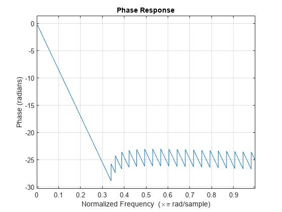
Use designfilt to design an FIR filter of order 54, normalized cutoff frequency $0.3 π$ rad/s, passband ripple 0.7 dB, and stopband attenuation 42 dB. Use the method of constrained least squares. Display the phase response of the filter.

Nf = 54;
Fc = 0.3;
Ap = 0.7;
As = 42;

d = designfilt('lowpassfir','CutoffFrequency',Fc,'FilterOrder',Nf, ...
               'PassbandRipple',Ap,'StopbandAttenuation',As, ...
               'DesignMethod','cls');
phasez(d)

Figure contains an axes object. The axes object with title Phase Response, xlabel Normalized Frequency ( times pi blank rad/sample), ylabel Phase (radians) contains an object of type line.

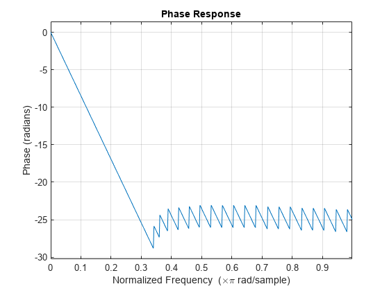
Design the same filter using fircls1. Keep in mind that fircls1 uses linear units to measure the ripple and attenuation.

pAp = 10^(Ap/40);
Apl = (pAp-1)/(pAp+1);

pAs = 10^(As/20);
Asl = 1/pAs;

b = fircls1(Nf,Fc,Apl,Asl);
phasez(b)

Figure contains an axes object. The axes object with title Phase Response, xlabel Normalized Frequency ( times pi blank rad/sample), ylabel Phase (radians) contains an object of type line.

Phase Response of an Equiripple Filter

Open Live Script

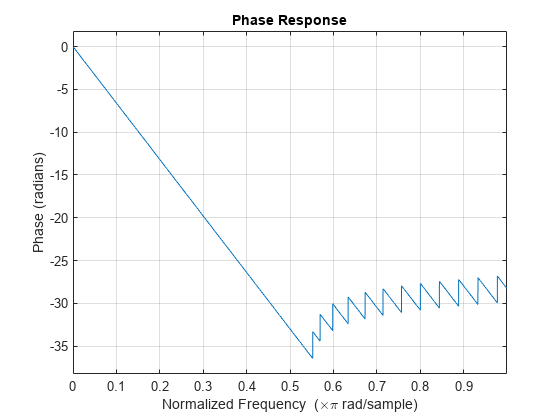
Design a lowpass equiripple filter with normalized passband frequency $0.45 π$ rad/s, normalized stopband frequency $0.55 π$ rad/s, passband ripple 1 dB, and stopband attenuation 60 dB. Display the phase response of the filter.

d = designfilt('lowpassfir', ...
               'PassbandFrequency',0.45,'StopbandFrequency',0.55, ...
               'PassbandRipple',1,'StopbandAttenuation',60, ...
               'DesignMethod','equiripple');
phasez(d)

Figure contains an axes object. The axes object with title Phase Response, xlabel Normalized Frequency ( times pi blank rad/sample), ylabel Phase (radians) contains an object of type line.

Phase Response of an Elliptic Filter

Open Live Script

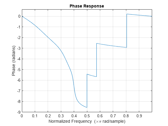
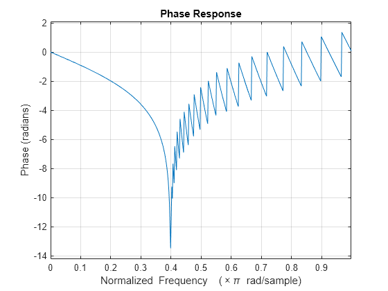
Design an elliptic lowpass IIR filter with normalized passband frequency $0.4 π$ rad/s, normalized stopband frequency $0.5 π$ rad/s, passband ripple 1 dB, and stopband attenuation 60 dB. Display the phase response of the filter.

d = designfilt('lowpassiir', ...
               'PassbandFrequency',0.4,'StopbandFrequency',0.5, ...
               'PassbandRipple',1,'StopbandAttenuation',60, ...
               'DesignMethod','ellip');
phasez(d)

Figure contains an axes object. The axes object with title Phase Response, xlabel Normalized Frequency ( times pi blank rad/sample), ylabel Phase (radians) contains an object of type line.

Phase Response from Cascaded Transfer Functions

Since R2024b

Open Live Script

Design a 40th-order lowpass Chebyshev type II digital filter with a stopband edge frequency of 0.4 and stopband attenuation of 50 dB. Plot the phase response of the filter using its coefficients in the CTF format.

[B,A] = cheby2(40,50,0.4,"ctf");

phasez(B,A,"ctf")

Figure contains an axes object. The axes object with title Phase Response, xlabel Normalized Frequency ( times pi blank rad/sample), ylabel Phase (radians) contains an object of type line.

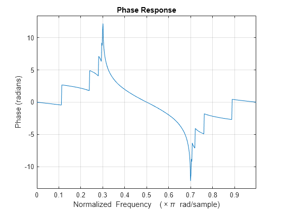
Design a 30th-order bandpass elliptic digital filter with passband edge frequencies of 0.3 and 0.7, passband ripple of 0.1 dB, and stopband attenuation of 50 dB. Plot the phase response of the filter using its coefficients and gain in the CTF format.

[B,A,g] = ellip(30,0.1,50,[0.3 0.7],"ctf");

phasez({B,A,g},"ctf")

Figure contains an axes object. The axes object with title Phase Response, xlabel Normalized Frequency ( times pi blank rad/sample), ylabel Phase (radians) contains an object of type line.

Input Arguments

`b`, `a` — Transfer function coefficients
vectors

Transfer function coefficients, specified as vectors. Express the transfer function in terms of b and a as

$H (z) = \frac{B (z)}{A (z)} = \frac{b_{1} + b_{2} z^{- 1} \dots + b_{n} z^{- (n - 1)} + b_{n + 1} z^{- n}}{a_{1} + a_{2} z^{- 1} \dots + a_{m} z^{- (m - 1)} + a_{m + 1} z^{- m}}$

Example: b = [1 3 3 1]/6 and a = [3 0 1 0]/3 specify a third-order Butterworth filter with normalized 3 dB frequency 0.5π rad/sample.

Data Types: double | single
Complex Number Support: Yes

`n` — Number of frequency points over which to evaluate response
512 (default) | positive integer scalar

Number of frequency points over which to evaluate response, specified as a positive integer scalar no less than 2. When n is absent, it defaults to 512. For best results, set n to a value greater than the filter order.

`B,A` — Cascaded transfer function (CTF) coefficients
scalars | vectors | matrices

Since R2024b

Cascaded transfer function (CTF) coefficients, specified as scalars, vectors, or matrices. B and A list the numerator and denominator coefficients of the cascaded transfer function, respectively.

B must be of size L-by-(m + 1) and A must be of size L-by-(n + 1), where:

L represents the number of filter sections.
m represents the order of the filter numerators.
n represents the order of the filter denominators.

For more information about the cascaded transfer function format and coefficient matrices, see Specify Digital Filters in CTF Format.

Note

If any element of A(:,1) is not equal to 1, then phasez normalizes the filter coefficients by A(:,1). In this case, A(:,1) must be nonzero.

Data Types: double | single
Complex Number Support: Yes

`g` — Scale values
scalar | vector

Since R2024b

Scale values, specified as a real-valued scalar or as a real-valued vector with L + 1 elements, where L is the number of CTF sections. The scale values represent the distribution of the filter gain across sections of the cascaded filter representation.

The phasez function applies a gain to the filter sections using the scaleFilterSections function depending on how you specify g:

Scalar — The function distributes the gain uniformly across all filter sections.
Vector — The function applies the first L gain values to the corresponding filter sections and distributes the last gain value uniformly across all filter sections.

Data Types: double | single

`d` — Digital filter
`digitalFilter` object

Digital filter, specified as a digitalFilter object. Use designfilt to generate a digital filter based on frequency-response specifications.

Example: d = designfilt('lowpassiir','FilterOrder',3,'HalfPowerFrequency',0.5) specifies a third-order Butterworth filter with normalized 3 dB frequency 0.5π rad/sample.

`sos` — Second-order section coefficients
matrix

Second-order section coefficients, specified as a matrix. sos is a K-by-6 matrix, where the number of sections, K, must be greater than or equal to 2. If the number of sections is less than 2, the function treats the input as a numerator vector. Each row of sos corresponds to the coefficients of a second-order (biquad) filter. The ith row of sos corresponds to [bi(1) bi(2) bi(3) ai(1) ai(2) ai(3)].

Example: s = [2 4 2 6 0 2;3 3 0 6 0 0] specifies a third-order Butterworth filter with normalized 3 dB frequency 0.5π rad/sample.

Data Types: double | single
Complex Number Support: Yes

`fs` — Sample rate
positive scalar

Sample rate, specified as a positive scalar. When the unit of time is seconds, fs is expressed in hertz.

Data Types: double

`w` — Angular frequencies
vector

Angular frequencies, specified as a vector and expressed in rad/sample. w must have at least two elements, because otherwise the function interprets it as n. w = π corresponds to the Nyquist frequency.

`f` — Frequencies
vector

Frequencies, specified as a vector. f must have at least two elements, because otherwise the function interprets it as n. When the unit of time is seconds, f is expressed in hertz.

Data Types: double

Output Arguments

`phi` — Phase response
vector

Phase response, returned as a vector. If you specify n, then phi has length n. If you do not specify n, or specify n as an empty vector, then phi has length 512.

If the input to phasez is single precision, the function computes the phase response using single-precision arithmetic. The output phi is single precision.

`w` — Angular frequencies
vector

Angular frequencies, returned as a vector. w has values ranging from 0 to π. If you specify 'whole' in your input, the values in w range from 0 to 2π. If you specify n, w has length n. If you do not specify n, or specify n as the empty vector, w has length 512.

`f` — Frequencies
vector

Frequencies, returned as a vector expressed in hertz. f has values ranging from 0 to fs/2 Hz. If you specify 'whole' in your input, the values in f range from 0 to fs Hz. If you specify n, f has length n. If you do not specify n, or specify n as an empty vector, f has length 512.

More About

Cascaded Transfer Functions

Partitioning an IIR digital filter into cascaded sections improves its numerical stability and reduces its susceptibility to coefficient quantization errors. The cascaded form of a transfer function H(z) in terms of the L transfer functions H₁(z), H₂(z), …, H_L(z) is

$H (z) = \prod_{l = 1}^{L} H_{l} (z) = H_{1} (z) \times H_{2} (z) \times \dots \times H_{L} (z) .$

Specify Digital Filters in CTF Format

You can specify digital filters in the CTF format for analysis, visualization, and signal filtering. Specify a filter by listing its coefficients B and A. You can also include the filter scaling gain across sections by specifying a scalar or vector g.

Filter Coefficients

When you specify the coefficients as L-row matrices,

$B = [\begin{matrix} b_{11} & b_{12} & \dots & b_{1, m + 1} \\ b_{21} & b_{22} & \dots & b_{2, m + 1} \\ ⋮ & ⋮ & ⋱ & ⋮ \\ b_{L 1} & b_{L 2} & \dots & b_{L, m + 1} \end{matrix}], A = [\begin{matrix} a_{11} & a_{12} & \dots & a_{1, n + 1} \\ a_{21} & a_{22} & \dots & a_{2, n + 1} \\ ⋮ & ⋮ & ⋱ & ⋮ \\ a_{L 1} & a_{L 2} & \dots & a_{L, n + 1} \end{matrix}],$

it is assumed that you have specified the filter as a sequence of L cascaded transfer functions, such that the full transfer function of the filter is

$H (z) = \frac{b_{11} + b_{12} z^{- 1} + \dots + b_{1, m + 1} z^{- m}}{a_{11} + a_{12} z^{- 1} + \dots + a_{1, n + 1} z^{- n}} \times \frac{b_{21} + b_{22} z^{- 1} + \dots + b_{2, m + 1} z^{- m}}{a_{21} + a_{22} z^{- 1} + \dots + a_{2, n + 1} z^{- n}} \times \dots \times \frac{b_{L 1} + b_{L 2} z^{- 1} + \dots + b_{L, m + 1} z^{- m}}{a_{L 1} + a_{L 2} z^{- 1} + \dots + a_{L, n + 1} z^{- n}},$

where m ≥ 0 is the numerator order of the filter and n ≥ 0 is the denominator order.

If you specify both B and A as vectors, it is assumed that the underlying system is a one-section IIR filter (L = 1), with B representing the numerator of the transfer function and A representing its denominator.
If B is scalar, it is assumed that the filter is a cascade of all-pole IIR filters with each section having an overall system gain equal to B.
If A is scalar, it is assumed that the filter is a cascade of FIR filters with each section having an overall system gain equal to 1/A.

Note

To convert second-order section matrices to cascaded transfer functions, use the sos2ctf function.
To convert a zero-pole-gain filter representation to cascaded transfer functions, use the zp2ctf function.

Coefficients and Gain

If you have an overall scaling gain or multiple scaling gains factored out from the coefficient values, you can specify the coefficients and gain as a cell array of the form {B,A,g}. Scaling filter sections is especially important when you work with fixed-point arithmetic to ensure that the output of each filter section has similar amplitude levels, which helps avoid inaccuracies in the filter response due to limited numeric precision.

The gain can be a scalar overall gain or a vector of section gains.

If the gain is scalar, the value applies uniformly to all the cascade filter sections.
If the gain is a vector, it must have one more element than the number of filter sections L in the cascade. Each of the first L scale values applies to the corresponding filter section, and the last value applies uniformly to all the cascade filter sections.

If you specify the coefficient matrices and gain vector as

$B = [\begin{matrix} b_{11} & b_{12} & \dots & b_{1, m + 1} \\ b_{21} & b_{22} & \dots & b_{2, m + 1} \\ ⋮ & ⋮ & ⋱ & ⋮ \\ b_{L 1} & b_{L 2} & \dots & b_{L, m + 1} \end{matrix}], A = [\begin{matrix} a_{11} & a_{12} & \dots & a_{1, n + 1} \\ a_{21} & a_{22} & \dots & a_{2, n + 1} \\ ⋮ & ⋮ & ⋱ & ⋮ \\ a_{L 1} & a_{L 2} & \dots & a_{L, n + 1} \end{matrix}], g = [\begin{matrix} g_{1} & g_{2} & \dots & g_{L} & g_{S} \end{matrix}],$

it is assumed that the transfer function of the filter system is

$H (z) = g_{S} (g_{1} \frac{b_{11} + b_{12} z^{- 1} + \dots + b_{1, m + 1} z^{- m}}{a_{11} + a_{12} z^{- 1} + \dots + a_{1, n + 1} z^{- n}} \times g_{2} \frac{b_{21} + b_{22} z^{- 1} + \dots + b_{2, m + 1} z^{- m}}{a_{21} + a_{22} z^{- 1} + \dots + a_{2, n + 1} z^{- n}} \times \dots \times g_{L} \frac{b_{L 1} + b_{L 2} z^{- 1} + \dots + b_{L, m + 1} z^{- m}}{a_{L 1} + a_{L 2} z^{- 1} + \dots + a_{L, n + 1} z^{- n}}) .$

Tips

You can obtain filters in CTF format, including the scaling gain. Use the outputs of digital IIR filter design functions, such as butter, cheby1, cheby2, and ellip. Specify the "ctf" filter-type argument in these functions and specify to return B, A, and g to get the scale values. (since R2024b)

References

[1] Lyons, Richard G. Understanding Digital Signal Processing. Upper Saddle River, NJ: Prentice Hall, 2004.

Extended Capabilities

C/C++ Code Generation
Generate C and C++ code using MATLAB® Coder™.

Usage notes and limitations:

If input b is a variable-sized matrix during code generation, then it must not reduce to a vector at runtime.
If input n is a variable-sized vector during code generation, then it must not reduce to a scalar at runtime.
If there is a discontinuity in the phase response, the result returned by the generated code might differ from the result returned by MATLAB^® by 2π.

Version History

Introduced before R2006a

R2024b: Analyze filters using cascaded transfer functions

The phasez function supports inputs in the cascaded transfer function (CTF) format.

See Also

Apps

Filter Analyzer | Filter Designer

Functions

ctffilt | designfilt | digitalFilter | freqz | phasedelay | grpdelay