ctffilt

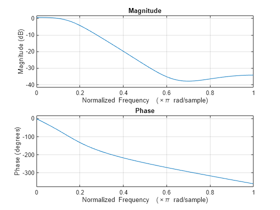
Specify a two-section digital filter with a transfer function $\mathit{H}\left(\mathit{z}\right)$. Plot the filter response.

B = [0.1607    0.2414    0.4689
     0.1607    0.0828    0.0551];
A = [     1         0         0;
          1   -1.1940    0.4360];
freqz(B,A,1024,"ctf")

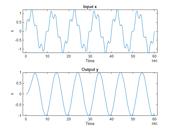
Filter a signal consisting of two sinusoidal waveforms with frequencies of 0.1 Hz and 0.45 Hz, sampled every half second over a duration of one minute. The amplitude of the 0.45 Hz waveform is 0.3 times the amplitude of the 0.1 Hz waveform.

t = (0:0.5:60)';
s = sin(2*pi*0.1*t)+0.3*sin(2*pi*0.45*t);

x = timetable(seconds(t),s);

y = ctffilt(B,A,x);

Compare the input and output signals in the time domain. Because the magnitude of the filter response at 0.1 Hz is 0 dB, the amplitude of the output signal y is as high as the amplitude of the 0.1 Hz waveform from the input signal x.

tiledlayout flow
nexttile
plot(x,"s")
title("Input x")
nexttile
plot(y,"s")
title("Output y")

Generate a sinusoidal signal with an amplitude of 1 V and a frequency of 60 Hz, and add third-, fifth-, and seventh-order harmonics. The harmonic amplitudes are 1 V, 0.1 V, and 0.03 V, respectively. Sample the signal for 1 second at a sample rate of 1000 Hz.

rng default
Fs = 1000;
a = [1 1 0.1 0.03];
f = 60*[1 3 5 7];
t = (0:1/Fs:1)';

x = cos(2*pi*f.*t)*a' + 0.005*randn(size(t));

Remove the third- and higher-order harmonic components from the mixed signal using a multisection lowpass elliptic filter. The cutoff frequency of the filter is 120 Hz.

Fc = 120;
wc = Fc/(Fs/2);
[num,den] = ellip(8,0.1,50,wc,"ctf");

y = ctffilt(num,den,x);

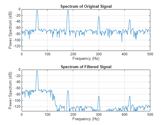
Plot the power spectrum for the original and filtered signals. The second plot shows that the power of the filtered signal decreases significantly at frequencies above 120 Hz.

tiledlayout flow
nexttile
pspectrum(x,Fs)
title("Spectrum of Original Signal")
ylim([-135 0])
nexttile
pspectrum(y,Fs)
title("Spectrum of Filtered Signal")
ylim([-135 0])

Design a fifth-order Butterworth bandpass filter represented as a cascade of fourth-order sections. The cutoff edge frequencies of the filter are 90 Hz and 150 Hz. The sample rate is 10 kHz.

Fs = 10000;
Wn  = [90 150]/(Fs/2);
[B,A] = butter(5,Wn,"bandpass","ctf")

B = 3×5

    0.0013    0.0026    0.0013         0         0
    0.0013    0.0026         0   -0.0026   -0.0013
    0.0013   -0.0052    0.0079   -0.0052    0.0013

A = 3×5

    1.0000   -1.9578    0.9630         0         0
    1.0000   -3.9289    5.7991   -3.8109    0.9408
    1.0000   -3.9650    5.9071   -3.9191    0.9770

The number of rows and columns in B and A indicate that the resulting filter has three fourth-order sections. There is one more column than the degree of the section polynomials to include the coefficient of the ${\mathit{z}}^0$ term.

Since the order of each filter section is four, the initial condition states in each section must have four elements. You can specify a four-element vector to set up the same initial condition states for the three filter sections, or a 12-element vector to set up these states explicitly for each filter section.

Specify the initial condition states for all filter sections as zeros.

L = size(B,1);
r = max(size(B,2),size(A,2))-1;
numStates = L*r;
zi = zeros(1,numStates);

Perform successive filtering on a noisy sinusoid using the bandpass filter.

rng default
t = single(0:1/Fs:1-1/Fs);
x = sin(2*pi*10*t) + 0.5*sin(2*pi*100*t) + 0.1*randn(size(t));
% Signal framing:
fl = 50; % Frame length
xFramed = framesig(x,fl);
% Successive filtering across frames:
ySuccessive = [];
zf = zi;
for nFrame = 1:size(xFramed,2)
    [yFrame,zf] = ctffilt(B,A,xFramed(:,nFrame)',zf);
    ySuccessive = [ySuccessive yFrame];
end

Filter the entire noisy signal in a single operation.

yDirect = ctffilt(B,A,x,zi);

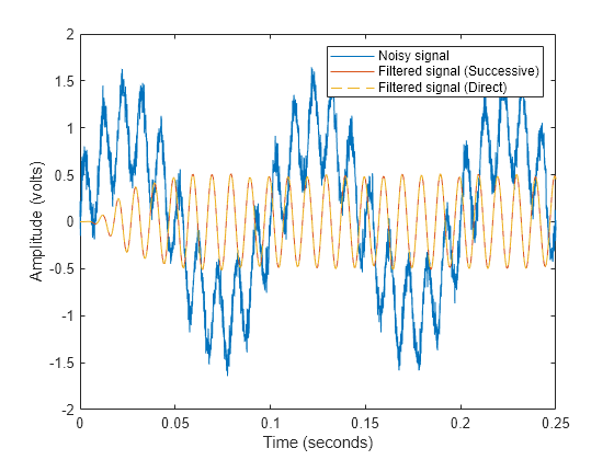
Compare the noisy signal with the filtered signal for the first 0.25 seconds. Successive filtering across the signal frames yields the same result as filtering the entire signal once.

plot(t,x,t,ySuccessive,t,yDirect,"--")
legend(["Noisy" "Filtered" "Filtered"]'+" signal" ...
    + ["" " (Successive)" " (Direct)"]')
xlabel("Time (seconds)")
ylabel("Amplitude (volts)")
xlim([0 0.25])

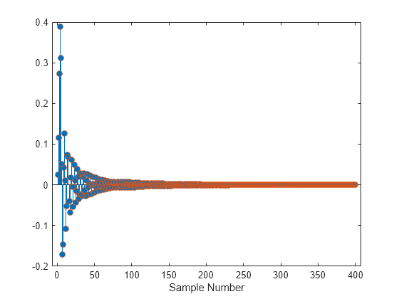
Design an eighth-order lowpass elliptic filter by specifying the sample rate ${\mathit{F}}_{\mathrm{s}}=8192$ Hz , cutoff frequency 2000 Hz, passband ripple 0.5 dB, and stopband attenuation 60 dB. Then, design an impulse signal with 400 samples.

% Filter design
Fs = 8192;
Wn = 2000/(Fs/2);
[num,den,sv] = ellip(8,0.5,60,Wn,"ctf");

% Impulse signal
Ns = 400;
x = [1;zeros(Ns-1,1)];

Derive the impulse response of the elliptic filter by filtering the impulse signal x and by computing the filter response.

% Filter impulse signal
h = ctffilt({num,den,sv},x);
% Compute filter impulse response
hImp = impz({num,den,sv},"ctf",Ns);

Compare the impulse responses. Both approaches yield the same result.

stem(h,"filled")
hold on
scatter(1:Ns,hImp)
hold off
xlabel("Sample Number")

Design a three-section decimate-by-five cascaded integrator-comb (CIC) filter. Each section has a unit differential delay. Plot the frequency response of the cascaded transfer function.

N = 1; % Differential delay
D = 5; % Decimation factor
K = 3; % Number of sections
num = repmat([1 zeros(1,N*D-1) -1],K,1)

num = 3×6

     1     0     0     0     0    -1
     1     0     0     0     0    -1
     1     0     0     0     0    -1

den = repmat([1 -1],K,1)

den = 3×2

     1    -1
     1    -1
     1    -1

freqz(num,den,"ctf")

Compute the 100-sample impulse and step responses of the CIC filter. Use the Dimension input argument to compute the filter responses using a multichannel signal structure x.

Ns = 100;
xImpl = [1 zeros(1,Ns-1)];
xStep = ones(1,Ns);
x = [xImpl;xStep];

y = ctffilt(num,den,x,Dimension=2);

Downsample and plot the decimated filter responses. Normalize the responses with respect to their maxima.

yDec = downsample(y',D);
plot(yDec./max(yDec),"*-")
xlabel("Sample Number")
title("Decimated Filter Responses")
legend(["Impulse" "Step"])