Wavelet Packet Harmonic Interference Removal

Wavelet Packet Transform and Baseline Shifting

In this example, we use a wavelet packet approach [3], which has the potential to be distortion free. See Wavelet Packets: Decomposing the Details for a review of the wavelet packet transform.

The basis of the wavelet packet technique for harmonic interference consists of the following steps:

The above method is based on the fact the detail subband coefficients in a wavelet packet transform are zero mean and the presence of a nonzero baseline in the resampled data indicates the presence of the harmonic interference.

60-Hz Interference Component

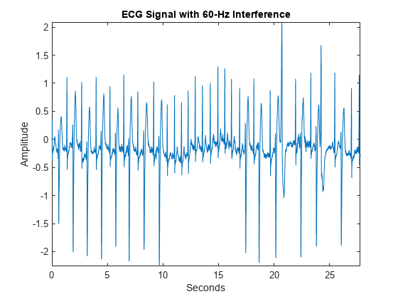
Load and plot an ECG signal corresponding to record 200 of the MIT-BIH Arrhythmia Database [1],[2]. The data is sampled at 360 Hz.

load mit200
plot(tm,ecgsig)
xlabel("Seconds")
ylabel("Amplitude")
axis tight
title("ECG Signal with 60-Hz Interference")

Plot the power spectrum of the data in order to clearly see the 60-Hz interference. Note this interference is not artificially injected in the data. It is present in the original recording.

pspectrum(ecgsig,360)
xlim([45 80])
title("Power Spectrum of ECG Signal with 60-Hz Interference")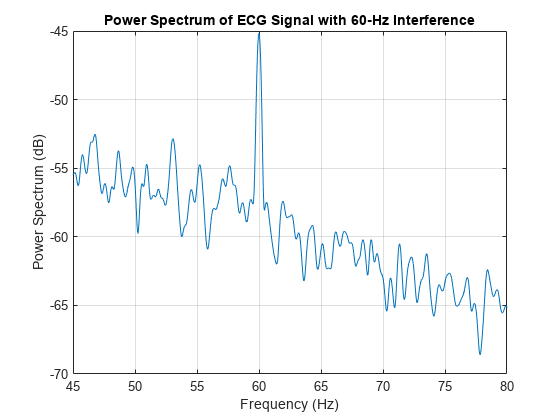

There is also a harmonic of 60 Hz visible in the data at 120 Hz. However, the level of that interference is approximately 20 dB below the level of the 60-Hz interference. Accordingly, we focus here on the 60-Hz component.

First, load and analyze two IIR notch filters designed using designNotchPeakIIR (DSP System Toolbox). The filters were designed with two Q factors, 35 and 100, with the default bandwidth of -3 dB.

load Q100Filter3
load Q35Filter3

Examine the magnitude and phase responses for the two filters with bandwidth levels of -3 dB.

helperFreqPhasePlot(Q100Filter3.num,Q100Filter3.den, ...
    Q35Filter3.num,Q35Filter3.den);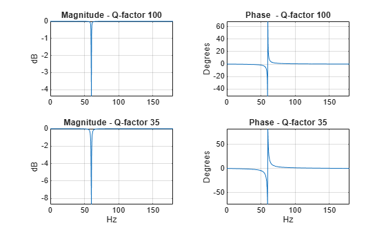

Zero-phase filter the ECG data using the notch filter with a Q-factor of 100. Plot the power spectrum of the filtered data.

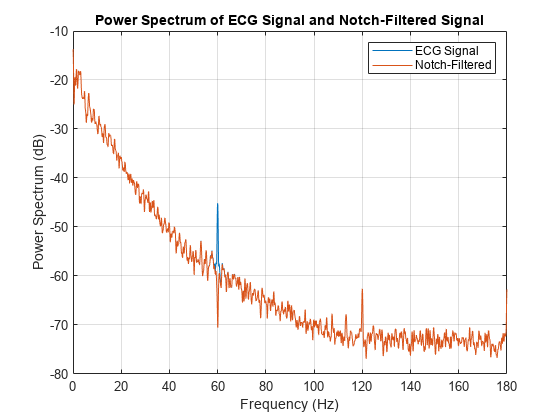
y = filtfilt(Q100Filter3.num,Q100Filter3.den,ecgsig);
figure
pspectrum([ecgsig,y],360)
xlim([55 65])
title("Power Spectrum of ECG Signal and Notch-Filtered Signal")
legend("ECG Signal", "Notch-Filtered")

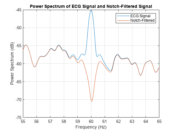
The notch filter has done a good job of removing the 60-Hz interference, but there is clearly some corruption of the signal's spectrum around the interference frequency.

If you zoom out to see the entire power spectrum from 0 to the Nyquist, the distortion of the signal's spectrum near 60 Hz is clearly visible, while overall the spectrum of the filtered signal matches the original signal's spectrum well.

xlim([0 180])

The helper function helperWPHarmonicFilter implements the baseline-shifted wavelet packet method described in [3]. Here we use the Daubechies least-asymmetric wavelet with 8 vanishing moments (16 coefficients).

sigWP = helperWPHarmonicFilter(ecgsig,60,"sym8",360,"reflection");
pspectrum([ecgsig,sigWP],360)
xlim([55 65])
title({"Power Spectrum of ECG Signal and" ; "Baseline-Shifted Wavelet Packet Signal"})
legend("ECG Signal","Wavelet Packet Cancellation",Location="SouthWest")

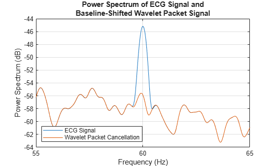
Note that the wavelet packet method has removed the harmonic interference without distorting the signal's spectrum around 60 hertz.

Zoom out to see the quality of the power spectrum for the wavelet packet method compared against the original signal from 0 to the Nyquist frequency.

xlim([0 180])

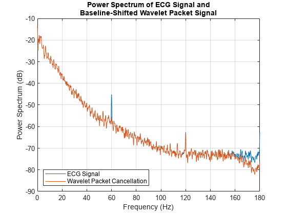
The overall spectrum of the wavelet packet method matches the signal spectrum quite well. There is some small distortion near the Nyquist. At this point, it is not clear if this due to the baseline-shifting algorithm or the resampling process. This warrants further investigation. However, there is no notable notch near the interference frequency as there is with the notch filter.

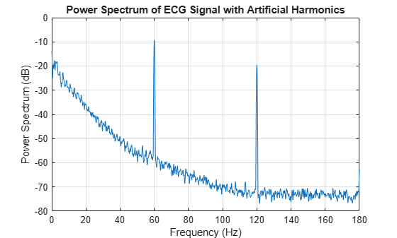
One of the advantages of the wavelet packet method is that it has the ability in theory to operate at multiple harmonics simultaneously. To illustrate this, load the signal ecgHarmonics. This is the mit200 signal with strong harmonic interference components injected at 60 and 120 Hz.

load ecgHarmonics
figure
pspectrum(ecgHarmonics,360)
title("Power Spectrum of ECG Signal with Artificial Harmonics")

Remove this harmonic interference using the wavelet packet method. Again, we use the Daubechies' least asymmetric phase wavelet with 8 vanishing moments.

sigWP = helperWPHarmonicFilter(ecgHarmonics,60,"sym8",360,"reflection");

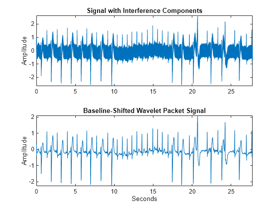
Plot the original signal and baseline-shifted wavelet packet reconstruction.

tiledlayout(2,1)
nexttile
plot(tm,ecgHarmonics)
ylabel("Amplitude")
axis tight
title("Signal with Interference Components")
nexttile
plot(tm,sigWP)
xlabel("Seconds")
ylabel("Amplitude")
title("Baseline-Shifted Wavelet Packet Signal")
axis tight

Examine the power spectra of both signals.

figure
pspectrum([ecgHarmonics,sigWP],360)
xlim([30 150])
title({"Power Spectrum of ECG Signal and" ; "Wavelet Packet Baseline-Shifted Signal"})
legend("ECG Signal with Interference","Baseline-Shifted Wavelet Packet Signal",Location="NorthEast")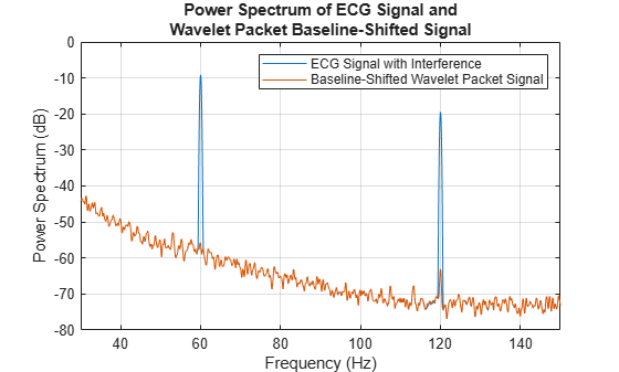

The result is quite good with both harmonics removed without spectral distortion in the neighborhood of the interference harmonics.

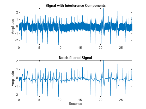
Compare this against IIR notch filtering. Here we need to filter the data twice, once for a notch filter operating at 60 Hz and once for a notch filter operating at 120 Hz. Alternatively, you can create a filter cascade. Here we want to use filtfilt for zero-phase filtering so we elect to implement the filtering twice.

Load the 120-Hz notch filter designed using designNotchPeakIIR with a Q factor of 100 and the default bandwidth level of -3 dB. Filter the signal first with the 60-Hz notch filter and then filter the output of that operation with the 120-Hz notch filter.

load Q100Filter3_120Hz
filt60Hz = filtfilt(Q100Filter3.num,Q100Filter3.den,ecgHarmonics);
filtCascade = filtfilt(Q100Filter3_120Hz.num,Q100Filter3_120Hz.den,filt60Hz);

Plot the original signal and notch-filtered signal.

tiledlayout(2,1)
nexttile
plot(tm,ecgHarmonics)
ylabel("Amplitude")
axis tight
title("Signal with Interference Components")
nexttile
plot(tm,filtCascade)
xlabel("Seconds")
ylabel("Amplitude")
title("Notch-filtered Signal")
axis tight

Examine the power spectra of both signals.

figure
pspectrum([ecgHarmonics,filtCascade],360)
xlim([30 150])
title("Power Spectrum of ECG Signal and Notch-filtered Signal")
legend("ECG Signal","Notch-Filtered Signal")

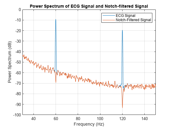
Here again we see distortion of the spectrum at the locations of the notch filters. Baseline shifting of the wavelet packet coefficients was more effective in removing the high-amplitude sinusoidal interference components.

Summary

This example looked at harmonic interference cancellation using the baseline-shifted wavelet packet technique described in [3]. In the ECG data considered here, the wavelet packet technique was effective at removing harmonic interference in both true and simulated conditions. The wavelet packet technique introduced less harmonic distortion in the signal's spectrum near the interference frequencies than notch filters. There was some distortion introduced by the wavelet packet technique near the Nyquist frequency, which warrants further investigation.

References

[1] Goldberger, Ary L., Luis A. N. Amaral, Leon Glass, Jeffrey M. Hausdorff, Plamen Ch. Ivanov, Roger G. Mark, Joseph E. Mietus, George B. Moody, Chung-Kang Peng, and H. Eugene Stanley. “PhysioBank, PhysioToolkit, and PhysioNet: Components of a New Research Resource for Complex Physiologic Signals.” Circulation 101, no. 23 (June 13, 2000). https://doi.org/10.1161/01.CIR.101.23.e215.

[2] Moody, G.B., and R.G. Mark. “The Impact of the MIT-BIH Arrhythmia Database.” IEEE Engineering in Medicine and Biology Magazine 20, no. 3 (June 2001): 45–50. https://doi.org/10.1109/51.932724.

[3] Lijun Xu. “Cancellation of Harmonic Interference by Baseline Shifting of Wavelet Packet Decomposition Coefficients.” IEEE Transactions on Signal Processing 53, no. 1 (January 2005): 222–30. https://doi.org/10.1109/TSP.2004.838954.

Helper Function

helperFreqPhasePlot

function helperFreqPhasePlot(num1,den1,num2,den2)
% This function is only intended to support this example. It may be
% changed or removed in a future release. 
figure
[H100,W] = freqz(num1,den1,[],360);
phi100 = phasez(num1,den1);
H35 = freqz(num2,den2,[],360);
phi35 = phasez(num2,den2);
tiledlayout(2,2)
nexttile
plot(W,10*log10(abs(H100)))
title("Magnitude - Q-factor 100")
ylabel("dB")
grid on
axis tight
nexttile
plot(W,phi100*180/pi)
title("Phase  - Q-factor 100")
ylabel("Degrees")
grid on
axis tight
nexttile
plot(W,10*log10(abs(H35)))
title("Magnitude - Q-factor 35")
xlabel("Hz")
ylabel("dB")
grid on
axis tight
nexttile
plot(W,phi35*180/pi)
title("Phase - Q-factor 35")
xlabel("Hz")
ylabel("Degrees")
grid on
axis tight


end