emd

Load and visualize a nonstationary continuous signal composed of sinusoidal waves with a distinct change in frequency. The vibration of a jackhammer and the sound of fireworks are examples of nonstationary continuous signals. The signal is sampled at a rate fs.

load("sinusoidalSignalExampleData.mat","X","fs")
t = (0:length(X)-1)/fs;

plot(t,X)
xlabel("Time (s)")

The mixed signal contains sinusoidal waves with different amplitude and frequency values.

To create the Hilbert spectrum plot, you need the intrinsic mode functions (IMFs) of the signal. Perform empirical mode decomposition to compute the IMFs and residuals of the signal. Since the signal is not smooth, specify 'pchip' as the interpolation method.

[imf,residual,info] = emd(X,Interpolation="pchip");

The table generated in the command window indicates the number of sift iterations, the relative tolerance, and the sift stop criterion for each generated IMF. This information is also contained in info. You can hide the table by adding the 'Display',0 name value pair.

Create the Hilbert spectrum plot using the imf components obtained using empirical mode decomposition.

hht(imf,fs)

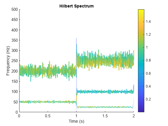
The frequency versus time plot is a sparse plot with a vertical color bar indicating the instantaneous energy at each point in the IMF. The plot represents the instantaneous frequency spectrum of each component decomposed from the original mixed signal. Three IMFs appear in the plot with a distinct change in frequency at 1 second.

This trigonometric identity presents two different views of the same physical signal:

$\frac{5}{2}\mathrm{cos2}\pi {\mathit{f}}_1\mathit{t}+\frac{1}{4}(\mathrm{cos2}\pi \left({\mathit{f}}_1+{\mathit{f}}_2\right)t+\mathrm{cos2}\pi \left({\mathit{f}}_1-{\mathit{f}}_2\right)t)=(2+{\cos }^2\pi {\mathit{f}}_2\mathit{t})\mathrm{cos2}\pi {\mathit{f}}_1\mathit{t}$.

Generate two sinusoids, s and z, such that s is the sum of three sine waves and z is a single sine wave with a modulated amplitude. Verify that the two signals are equal by calculating the infinity norm of their difference.

t = 0:1e-3:10;
omega1 = 2*pi*100;
omega2 = 2*pi*20;
s = 0.25*cos((omega1-omega2)*t) + ...
    2.5*cos(omega1*t) + ...
    0.25*cos((omega1+omega2)*t);
z = (2+cos(omega2/2*t).^2).*cos(omega1*t);

norm(s-z,Inf) 

ans = 
3.2729e-13

Plot the sinusoids and select a 1-second interval starting at 2 seconds.

plot(t,[s' z'])
xlim([2 3])
xlabel('Time (s)')
ylabel('Signal')

Obtain the spectrogram of the signal. The spectrogram shows three distinct sinusoidal components. Fourier analysis sees the signals as a superposition of sine waves.

pspectrum(s,1000,'spectrogram','TimeResolution',4)

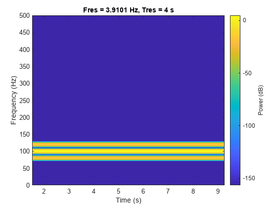
Use emd to compute the intrinsic mode functions (IMFs) of the signal and additional diagnostic information. The function by default outputs a table that indicates the number of sifting iterations, the relative tolerance, and the sifting stop criterion for each IMF. Empirical mode decomposition sees the signal as z.

[imf,~,info] = emd(s);

The number of zero crossings and local extrema differ by at most one. This satisfies the necessary condition for the signal to be an IMF.

info.NumZerocrossing - info.NumExtrema

ans = 
1

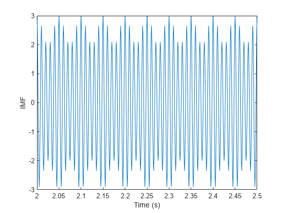
Plot the IMF and select a 0.5-second interval starting at 2 seconds. The IMF is an AM signal because emd views the signal as amplitude modulated.

plot(t,imf)
xlim([2 2.5])
xlabel('Time (s)')
ylabel('IMF')

Simulate a vibration signal from a damaged bearing. Perform empirical mode decomposition to visualize the IMFs of the signal and look for defects.

A bearing with a pitch diameter of 12 cm has eight rolling elements. Each rolling element has a diameter of 2 cm. The outer race remains stationary as the inner race is driven at 25 cycles per second. An accelerometer samples the bearing vibrations at 10 kHz.

fs = 10000;
f0 = 25;
n = 8;
d = 0.02;
p = 0.12;

The vibration signal from the healthy bearing includes several orders of the driving frequency.

t = 0:1/fs:10-1/fs;
a = 0.2*[1 0.5 0.2 0.1 0.05];
f = f0*[1 2 3 4 5];
yHealthy = a*sin(2*pi*f'.*t);

A resonance is excited in the bearing vibration halfway through the measurement process.

yHealthy = (1+1./(1+linspace(-10,10,length(yHealthy)).^4)).*yHealthy;

The resonance introduces a defect in the outer race of the bearing that results in progressive wear. The defect causes a series of impacts that recur at the ball pass frequency outer race (BPFO) of the bearing:

where $$f_0$$ is the driving rate, $$n$$ is the number of rolling elements, $$d$$ is the diameter of the rolling elements, $$p$$ is the pitch diameter of the bearing, and $$\theta$$ is the bearing contact angle. Assume a contact angle of 15° and compute the BPFO.

ca = 15;
bpfo = n*f0/2*(1-d/p*cosd(ca));

Use the pulstran (Signal Processing Toolbox) function to model the impacts as a periodic train of 5-millisecond sinusoids. Each 3 kHz sinusoid is windowed by a flat top window. Use a power law to introduce progressive wear in the bearing vibration signal.

fImpact = 3000;
tImpact = 0:1/fs:5e-3-1/fs;
wImpact = flattopwin(length(tImpact))'/10;
xImpact = sin(2*pi*fImpact*tImpact).*wImpact;

tx = 0:1/bpfo:t(end);
tx = [tx; 1.3.^tx-2];

nWear = 49000;
nSamples = 100000;
yImpact = pulstran(t,tx',xImpact,fs)/5;
yImpact = [zeros(1,nWear) yImpact(1,(nWear+1):nSamples)];

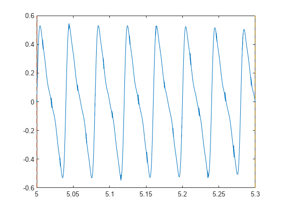
Generate the BPFO vibration signal by adding the impacts to the healthy signal. Plot the signal and select a 0.3-second interval starting at 5.0 seconds.

yBPFO = yImpact + yHealthy;

xLimLeft = 5.0;
xLimRight = 5.3;
yMin = -0.6;
yMax = 0.6;

plot(t,yBPFO)

hold on
[limLeft,limRight] = meshgrid([xLimLeft xLimRight],[yMin yMax]);
plot(limLeft,limRight,"--")
hold off
xlabel("Time (seconds)")
ylabel("Amplitude")

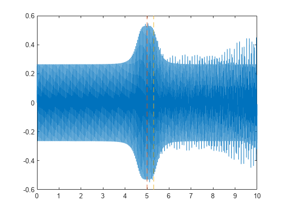
Zoom in on the selected interval to visualize the effect of the impacts.

xlim([xLimLeft xLimRight])

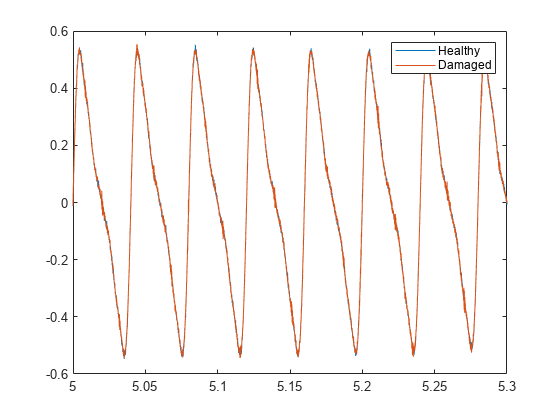
Add white Gaussian noise to the signals. Specify a noise variance of $$1/150^2$$.

rn = 150;
yGood = yHealthy + randn(size(yHealthy))/rn;
yBad = yBPFO + randn(size(yHealthy))/rn;

plot(t,yGood,t,yBad)
xlim([xLimLeft xLimRight])
legend("Healthy","Damaged")
xlabel("Time (seconds)")
ylabel("Amplitude")

Use emd to perform an empirical mode decomposition of the healthy bearing signal. Compute the first five intrinsic mode functions (IMFs). Use the Display name-value argument to show a table with the number of sifting iterations, the relative tolerance, and the sifting stop criterion for each IMF.

imfGood = emd(yGood,MaxNumIMF=5,Display=1);

Current IMF  |  #Sift Iter  |  Relative Tol  |  Stop Criterion Hit  
      1      |        3     |     0.017132   |  SiftMaxRelativeTolerance
      2      |        3     |      0.12694   |  SiftMaxRelativeTolerance
      3      |        6     |      0.14582   |  SiftMaxRelativeTolerance
      4      |        1     |     0.011082   |  SiftMaxRelativeTolerance
      5      |        2     |      0.03463   |  SiftMaxRelativeTolerance
Decomposition stopped because maximum number of intrinsic mode functions was extracted.

Use emd without output arguments to visualize the first three modes and the residual.

emd(yGood,MaxNumIMF=5)

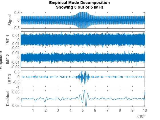
Compute and visualize the IMFs of the defective bearing signal. The first empirical mode reveals the high-frequency impacts. This high-frequency mode increases in energy as the wear progresses. The third mode shows the resonance in the vibration signal.

imfBad = emd(yBad,MaxNumIMF=5,Display=1);

Current IMF  |  #Sift Iter  |  Relative Tol  |  Stop Criterion Hit  
      1      |        2     |     0.041274   |  SiftMaxRelativeTolerance
      2      |        3     |      0.16695   |  SiftMaxRelativeTolerance
      3      |        3     |      0.18428   |  SiftMaxRelativeTolerance
      4      |        1     |     0.037177   |  SiftMaxRelativeTolerance
      5      |        2     |     0.095861   |  SiftMaxRelativeTolerance
Decomposition stopped because maximum number of intrinsic mode functions was extracted.

emd(yBad,MaxNumIMF=5)

The next step in the analysis is to compute the Hilbert spectrum of the extracted IMFs. For more details, see the Compute Hilbert Spectrum of Vibration Signal (Signal Processing Toolbox) example.

Load and visualize a nonstationary continuous signal composed of sinusoidal waves with a distinct change in frequency. The vibration of a jackhammer and the sound of fireworks are examples of nonstationary continuous signals. The signal is sampled at a rate fs.

load("sinusoidalSignalExampleData.mat","X","fs")
t = (0:length(X)-1)/fs;
plot(t,X)
xlabel("Time(s)")

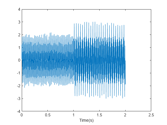
The mixed signal contains sinusoidal waves with different amplitude and frequency values.

Perform empirical mode decomposition to plot the intrinsic mode functions and residual of the signal. Since the signal is not smooth, specify "pchip" as the interpolation method.

emd(X,Interpolation="pchip",Display=1)

Current IMF  |  #Sift Iter  |  Relative Tol  |  Stop Criterion Hit  
      1      |        2     |     0.026352   |  SiftMaxRelativeTolerance
      2      |        2     |    0.0039573   |  SiftMaxRelativeTolerance
      3      |        1     |     0.024838   |  SiftMaxRelativeTolerance
      4      |        2     |      0.05929   |  SiftMaxRelativeTolerance
      5      |        2     |      0.11317   |  SiftMaxRelativeTolerance
      6      |        2     |      0.12599   |  SiftMaxRelativeTolerance
      7      |        2     |      0.13802   |  SiftMaxRelativeTolerance
      8      |        3     |      0.15937   |  SiftMaxRelativeTolerance
      9      |        2     |      0.15923   |  SiftMaxRelativeTolerance
Decomposition stopped because the number of extrema in the residual signal is less than the 'MaxNumExtrema' value.

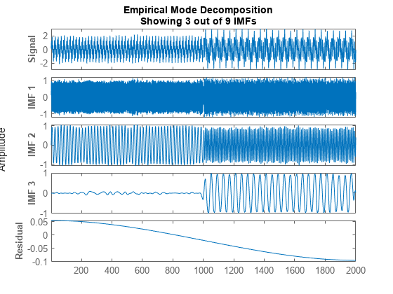
emd generates an interactive figure with the original signal, the first 3 IMFs, and the residual. The table generated in the command window indicates the number of sift iterations, the relative tolerance, and the sift stop criterion for each generated IMF. You can hide the table by removing the Display name-value argument or specifying it as 0.

Right-click on the white space in the figure to open the IMF selector window. Use IMF selector to selectively view the generated IMFs, the original signal, and the residual.

Select the IMFs to be displayed from the list. Choose whether to display the original signal and residual on the figure.

The selected IMFs are now displayed on the figure.

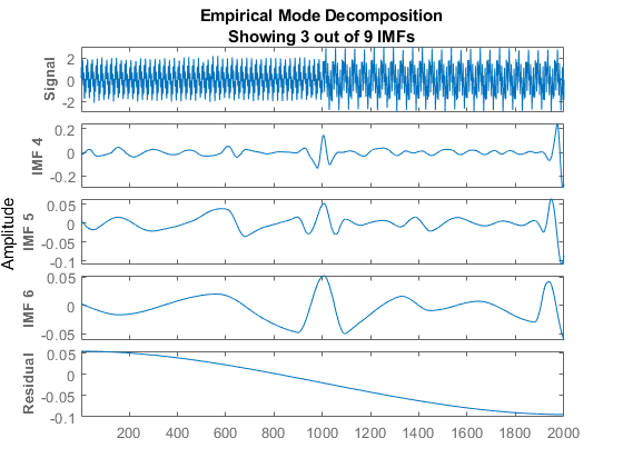
Use the figure to visualize individual components decomposed from the original signal along with the residual. Note that the residual is computed for the total number of IMFs, and does not change based on the IMFs selected in the IMF selector window.

References

[1] Huang, Norden E., Zheng Shen, Steven R. Long, Manli C. Wu, Hsing H. Shih, Quanan Zheng, Nai-Chyuan Yen, Chi Chao Tung, and Henry H. Liu. “The Empirical Mode Decomposition and the Hilbert Spectrum for Nonlinear and Non-Stationary Time Series Analysis.” Proceedings of the Royal Society of London. Series A: Mathematical, Physical and Engineering Sciences 454, no. 1971 (March 8, 1998): 903–95. https://doi.org/10.1098/rspa.1998.0193.
[2] Rato, R.T., M.D. Ortigueira, and A.G. Batista. “On the HHT, Its Problems, and Some Solutions.” Mechanical Systems and Signal Processing 22, no. 6 (August 2008): 1374–94. https://doi.org/10.1016/j.ymssp.2007.11.028.
[3] Rilling, Gabriel, Patrick Flandrin, and Paulo Gonçalves. "On Empirical Mode Decomposition and Its Algorithms." IEEE-EURASIP Workshop on Nonlinear Signal and Image Processing 2003. NSIP-03. Grado, Italy. 8–11.
[4] Wang, Gang, Xian-Yao Chen, Fang-Li Qiao, Zhaohua Wu, and Norden E. Huang. “On Intrinsic Mode Function.” Advances in Adaptive Data Analysis 02, no. 03 (July 2010): 277–93. https://doi.org/10.1142/S1793536910000549.
Extended Capabilities
Usage notes and limitations:
Timetables are not supported for code generation.
If supplied, the interpolation method specified using the
'Interpolation'name-value pair must be a compile-time constant.
Refer to the usage notes and limitations in the C/C++ Code Generation section. The same usage notes and limitations apply to GPU code generation.
Version History
Introduced in R2018a
MATLAB Command
You clicked a link that corresponds to this MATLAB command:
Run the command by entering it in the MATLAB Command Window. Web browsers do not support MATLAB commands.
选择网站
选择网站以获取翻译的可用内容,以及查看当地活动和优惠。根据您的位置,我们建议您选择:。
您也可以从以下列表中选择网站:
如何获得最佳网站性能
选择中国网站(中文或英文)以获得最佳网站性能。其他 MathWorks 国家/地区网站并未针对您所在位置的访问进行优化。
美洲
- América Latina (Español)
- Canada (English)
- United States (English)
欧洲
- Belgium (English)
- Denmark (English)
- Deutschland (Deutsch)
- España (Español)
- Finland (English)
- France (Français)
- Ireland (English)
- Italia (Italiano)
- Luxembourg (English)
- Netherlands (English)
- Norway (English)
- Österreich (Deutsch)
- Portugal (English)
- Sweden (English)
- Switzerland
- United Kingdom (English)