vmd

Variational mode decomposition

Since R2020a

collapse all in page

Syntax

imf = vmd(x)

[imf,residual] = vmd(x)

[imf,residual,info] = vmd(x)

[___] = vmd(x,Name=Value)

vmd(___)

Description

imf = vmd(x) returns the variational mode decomposition of x. Use vmd to decompose and simplify complicated signals into a finite number of intrinsic mode functions (IMFs) required to perform Hilbert spectral analysis.

example

[imf,residual] = vmd(x) also returns the residual signal residual corresponding to the variational mode decomposition of x.

[imf,residual,info] = vmd(x) returns additional information info on IMFs and the residual signal for diagnostic purposes.

example

[___] = vmd(x,Name=Value) performs the variational mode decomposition with additional options specified by one or more name-value arguments.

example

vmd(___) plots the original signal, IMFs, and the residual signal as subplots in the same figure.

example

Examples

collapse all

Variational Mode Decomposition of Dial Tone Signal

Open Live Script

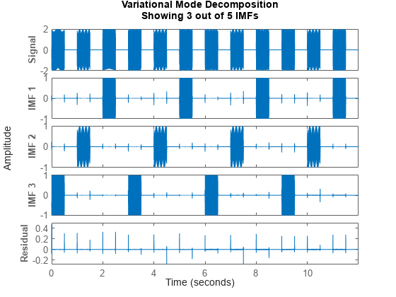
Create a signal, sampled at 4 kHz, that resembles dialing all the keys of a digital telephone. Save the signal as a MATLAB® timetable.

fs = 4e3;
t = 0:1/fs:0.5-1/fs;

ver = [697 770 852 941];
hor = [1209 1336 1477];

tones = [];

for k = 1:length(ver)
    for l = 1:length(hor)
        tone = sum(sin(2*pi*[ver(k);hor(l)].*t))';
        tones = [tones;tone;zeros(size(tone))];
    end
end

% To hear, type soundsc(tones,fs)

S = timetable(tones,'SampleRate',fs);

Plot the variational mode decomposition of the timetable.

vmd(S)

VMD of Multicomponent Signal

Open Live Script

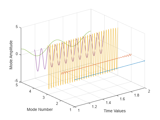
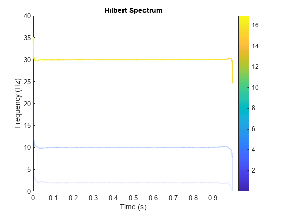
Generate a multicomponent signal consisting of three sinusoids of frequencies 2 Hz, 10 Hz, and 30 Hz. The sinusoids are sampled at 1 kHz for 2 seconds. Embed the signal in white Gaussian noise of variance 0.01².

fs = 1e3;
t = 1:1/fs:2-1/fs;
x = cos(2*pi*2*t) + ...
    2*cos(2*pi*10*t) + ...
    4*cos(2*pi*30*t) + ...
    0.01*randn(1,length(t));

Compute the IMFs of the noisy signal and visualize them in a 3-D plot.

imf = vmd(x);
[p,q] = ndgrid(t,1:size(imf,2));
plot3(p,q,imf)
grid on
xlabel('Time Values')
ylabel('Mode Number')
zlabel('Mode Amplitude')

Figure contains an axes object. The axes object with xlabel Time Values, ylabel Mode Number contains 5 objects of type line.

Use the computed IMFs to plot the Hilbert spectrum of the multicomponent signal. Restrict the frequency range to [0, 40] Hz.

hht(imf,fs,'FrequencyLimits',[0,40])

Figure contains an axes object. The axes object with title Hilbert Spectrum, xlabel Time (s), ylabel Frequency (Hz) contains 5 objects of type patch.

VMD of Piecewise Signal

Open Live Script

Generate a piecewise composite signal consisting of a quadratic trend, a chirp, and a cosine with a sharp transition between two constant frequencies at t = 0.5.

$x (t) = 6 t^{2} + \cos (4 π t + 10 π t^{2}) + {\begin{cases} \cos (60 π t), & t \leq 0.5, \\ \cos (100 π t - 10 π), & t > 0.5 . \end{cases}$

The signal is sampled at 1 kHz for 1 second. Plot each individual component and the composite signal.

fs = 1e3;
t = 0:1/fs:1-1/fs;

x = 6*t.^2 + cos(4*pi*t+10*pi*t.^2) + ...
    [cos(60*pi*(t(t<=0.5))) cos(100*pi*(t(t>0.5)-10*pi))];

tiledlayout('flow')
nexttile
plot(t,[zeros(1,length(t)/2) cos(100*pi*(t(length(t)/2+1:end))-10*pi)])
xlabel('Time (s)')
ylabel('Cosine')

nexttile
plot(t,[cos(60*pi*(t(1:length(t)/2))) zeros(1,length(t)/2)])
xlabel('Time (s)')
ylabel('Cosine')

nexttile
plot(t,cos(4*pi*t+10*pi*t.^2))
xlabel('Time (s)')
ylabel('Chirp')


nexttile
plot(t,6*t.^2)
xlabel('Time (s)')
ylabel('Quadratic trend')

nexttile(5,[1 2])
plot(t,x)
xlabel('Time (s)')
ylabel('Signal')

Perform variational mode decomposition to compute four intrinsic mode functions. The four distinct components of the signal are recovered.

[imf,res] = vmd(x,'NumIMFs',4);

tiledlayout('flow')

for i = 1:4
    nexttile
    plot(t,imf(:,i))
    txt = ['IMF',num2str(i)];
    ylabel(txt)
    xlabel('Time (s)')
    grid on
end

Reconstruct the signal by adding the mode functions and the residual. Plot and compare the original and reconstructed signals.

sig = sum(imf,2) + res;

nexttile(5,[1 2])
plot(t,sig,'LineWidth',1.5)

hold on

plot(t,x,':','LineWidth',2)
xlabel('Time (s)')
ylabel('Signal')
hold off
legend('Reconstructed signal','Original signal', ...
       'Location','northwest')

Calculate the norm of the difference between the original and the reconstructed signals.

norm(x-sig',Inf)

ans = 
0

Noise Removal from ECG Signal Using VMD

Open Live Script

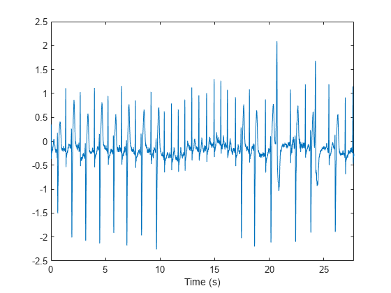
Load a signal corresponding to record 200 of the MIT-BIH Arrhythmia Database [3] (Signal Processing Toolbox). The signal was sampled at 360 Hz. Plot the signal.

load mit200

plot(tm,ecgsig)
xlabel("Time (s)")
xlim([tm(1) tm(end)])

Figure contains an axes object. The axes object with xlabel Time (s) contains an object of type line.

The ECG signal contains spikes driven by the rhythm of the heartbeat and an oscillating low-frequency pattern. The distinct spikes of the ECG create important higher-order harmonics.

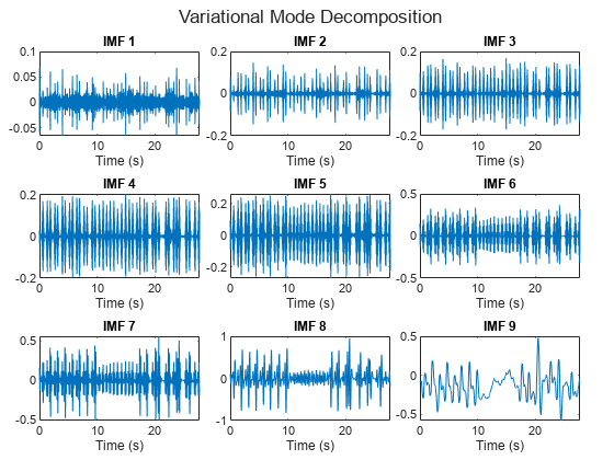
Calculate nine intrinsic mode functions of the windowed signal. Visualize the IMFs.

[imf,residual] = vmd(ecgsig,NumIMFs=9);

t = tiledlayout(3,3, ...
    TileSpacing="compact",Padding="compact");
for n = 1:9
    nexttile(t)
    plot(tm,imf(:,n))
    xlim([tm(1) tm(end)])
    title("IMF "+n)
    xlabel("Time (s)")
end
title(t,"Variational Mode Decomposition")

Construct a clean ECG signal by summing all the VMD modes except for the first, which contains most of the high-frequency noise, and the last, which contains the low-frequency baseline oscillation.

cleanECG = sum(imf(:,2:8),2);

figure
plot(tm,ecgsig,":",tm,cleanECG)
legend("Original ECG","Clean ECG")
xlabel("Time (s)")
xlim([tm(1) tm(end)])

Figure contains an axes object. The axes object with xlabel Time (s) contains 2 objects of type line. These objects represent Original ECG, Clean ECG.

Input Arguments

collapse all

`x` — Uniformly sampled time-domain signal
vector | timetable

Uniformly sampled time-domain signal, specified as either a vector or a timetable. If x is a timetable, then it must contain increasing finite row times. The timetable must contain only one numeric data vector with finite load values.

Note

If a timetable has missing or duplicate time points, you can fix it using the tips in Clean Timetable with Missing, Duplicate, or Nonuniform Times.

Name-Value Arguments

Specify optional pairs of arguments as Name1=Value1,...,NameN=ValueN, where Name is the argument name and Value is the corresponding value. Name-value arguments must appear after other arguments, but the order of the pairs does not matter.

Before R2021a, use commas to separate each name and value, and enclose Name in quotes.

Example: 'NumIMFs',10

`AbsoluteTolerance` — Mode convergence absolute tolerance
`5e-6` (default) | positive real scalar

Mode convergence absolute tolerance, specified as a positive real scalar. AbsoluteTolerance is one of the stopping criteria for optimization, that is, optimization stops when the average squared absolute improvement toward convergence of IMFs, in two consecutive iterations, is less than AbsoluteTolerance.

`RelativeTolerance` — Mode convergence relative tolerance
`AbsoluteTolerance*1e3` (default) | positive real scalar

Mode convergence relative tolerance, specified as a positive real scalar. RelativeTolerance is one of the stopping criteria for optimization, that is, optimization stops when the average relative improvement toward convergence of IMFs, in two consecutive iterations, is less than RelativeTolerance.

Note

The optimization process stops when AbsoluteTolerance and RelativeTolerance are jointly satisfied.

`MaxIterations` — Maximum number of optimization iterations
`500` (default) | positive scalar integer

Maximum number of optimization iterations, specified as a positive scalar integer. MaxIterations is one of the stopping criteria for optimization, that is, optimization stops when the number of iterations is greater than MaxIterations.

MaxIterations can be specified using only positive whole numbers.

`NumIMFs` — Number of IMFs extracted
`5` (default) | positive scalar integer

Number of IMFs extracted, specified as a positive scalar integer.

`CentralFrequencies` — Initial central IMF frequencies
vector

Initial central IMF frequencies, specified as a vector of length NumIMFs. Vector values must be within [0, 0.5] cycles/sample, which indicates that the true frequencies are within [0, f_s/2], where f_s is the sample rate.

`InitialIMFs` — Initial IMFs
zero matrix (default) | real matrix

Initial IMFs, specified as a real matrix. The rows correspond to time samples and columns correspond to modes.

`PenaltyFactor` — Penalty factor
`1000` (default) | positive real scalar

Penalty factor, specified as a positive real scalar. This argument determines the reconstruction fidelity. Use smaller values of penalty factor to obtain stricter data fidelity.

`InitialLM` — Initial Lagrange multiplier
complex vector of zeros (default) | complex vector

Initial Lagrange multiplier, specified as a complex vector. The range of the initial Lagrange multiplier in the frequency domain is [0, 0.5] cycles/sample. The multiplier enforces the reconstruction constraint. The length of the multiplier depends on the input size.

`LMUpdateRate` — Update rate for Lagrange multiplier
`0.01` (default) | real scalar

Update rate for the Lagrange multiplier in each iteration, specified as a positive real scalar. A higher rate results in faster convergence, but increases the chance of the optimization process getting stuck in a local optimum.

`InitializeMethod` — Method to initialize central frequencies
`"peaks"` (default) | `"random"` | `"grid"`

Method to initialize the central frequencies, specified as "peaks", "random", or "grid".

"peaks" — Initialize the central frequencies as the peak locations of the signal in the frequency domain (default). If NumIMFs (Signal Processing Toolbox) is greater than the number of frequency-domain peaks, vmd initializes the remaining central frequencies at random.
"random" — Initialize the central frequencies as random numbers distributed uniformly in the interval [0,0.5] cycles/sample.
"grid" — Initialize the central frequencies as a uniformly sampled grid in the interval [0,0.5] cycles/sample.

`Display` — Toggle progress display in command window
`false` or 0 (default) | `true` or 1

Toggle progress display in the command window, specified as either "true" (or 1) or "false" (or 0). If you specify "true", the function displays the average absolute and relative improvement of modes and central frequencies every 20 iterations, and shows the final stopping information.

Specify Display as 1 to show the table or 0 to hide the table.

Output Arguments

collapse all

`imf` — Intrinsic mode function
matrix | timetable

Intrinsic mode functions, returned as a matrix or timetable. Each imf is an amplitude and frequency modulated signal with positive and slowly varying envelopes. Each mode has an instantaneous frequency that is nondecreasing, varies slowly, and is concentrated around a central value. Use imf to apply Hilbert-Huang transform to perform spectral analysis on the signal.

imf is returned as:

A matrix where each column is an imf, when x is a vector.
A timetable, when x is a single data column timetable.

`residual` — Residual signal
column vector | single data column timetable

Residual signal, returned as a column vector or a single data column timetable. residual represents the portion of the original signal x not decomposed by vmd.

residual is returned as:

A column vector, when x is a vector.
A single data column timetable, when x is a single data column timetable.

`info` — Additional information for diagnostics
structure

Additional information for diagnostics, returned as a structure with these fields:

ExitFlag – Termination flag. A value of 0 indicates the algorithm stopped when it reached the maximum number of iterations. A value of 1 indicates the algorithm stopped when it met the absolute and relative tolerances.
CentralFrequencies – Central frequencies of the IMFs.
NumIterations – Total number of iterations.
AbsoluteImprovement – Average squared absolute improvement toward convergence of the IMFs between the final two iterations.
RelativeImprovement – Average relative improvement toward convergence of the IMFs between the final two iterations.
LagrangeMultiplier – Frequency-domain Lagrange multiplier at the last iteration.

More About

collapse all

Intrinsic Mode Functions

The vmd function decomposes a signal x(t) into a small number K of narrowband intrinsic mode functions (IMFs):

$x (t) = \sum_{k = 1}^{K} u_{k} (t) .$

The IMFs have these characteristics:

Each mode u_k is an amplitude and frequency modulated signal of the form

$u_{k} (t) = A_{k} (t) \cos (ϕ_{k} (t)),$
where ϕ_k(t) is the phase of the mode and A_k(t) is its envelope.
The modes have positive and slowly varying envelopes.
Each mode has an instantaneous frequency ϕ'_k(t) that is nondecreasing, varies slowly, and is concentrated around a central value f_k.

The variational mode decomposition method simultaneously calculates all the mode waveforms and their central frequencies. The process consists of finding a set of u_k(t) and f_k(t) that minimize the constrained variational problem.

Optimization

To calculate u_k and f_k, the procedure finds an optimum of the augmented Lagrangian

$\begin{matrix} L (u_{k} (t), f_{k}, λ (t)) & = & α \sum_{k = 1}^{K} {‖ \frac{d}{d t} [(δ (t) + \frac{j}{π t}) * u_{k} (t)] e^{- j 2 π f_{k} t} ‖}_{2}^{2} & + & {‖ x (t) - \sum_{k = 1}^{K} u_{k} (t) ‖}_{2}^{2} & + & 〈 λ (t), x (t) - \sum_{k = 1}^{K} u_{k} (t) 〉 \\ (i) & (i i) & (i i i) \end{matrix},$

where the inner product $〈 p (t), q (t) 〉 = \int_{- \infty}^{\infty} p^{*} (t) q (t) d t$ and the 2-norm ${‖ p (t) ‖}_{2}^{2} = 〈 p (t), p (t) 〉$ . The regularization term (i) includes these steps:

Use the Hilbert transform to calculate the analytic signal associated with each mode, where * denotes convolution. This results in each mode having a purely positive spectrum.
Demodulate the analytic signal to baseband by multiplying it with a complex exponential.
Estimate the bandwidth by calculating the squared 2-norm of the gradient of the demodulated analytic signal.

Terms (ii) and (iii) enforce the constraint $x (t) = \sum_{k = 1}^{K} u_{k} (t)$ by imposing a quadratic penalty and incorporating a Lagrange multiplier. The PenaltyFactor α measures the relative importance of (i) compared to (ii) and (iii).

The algorithm solves the optimization problem using the alternating direction method of multipliers described in [1] (Signal Processing Toolbox).

Algorithms

The vmd function calculates the IMFs in the frequency domain, reconstructing X(f) = DFT{x(t)} in terms of U_k(f) = DFT{u_k(t)}. To remove edge effects, the algorithm extends the signal by mirroring half its length on either side.

The Lagrange multiplier introduced in Optimization (Signal Processing Toolbox) has the Fourier transform Ʌ(f). The length of the Lagrange multiplier vector is the length of the extended signal.

Unless otherwise specified in InitialIMFs, the IMFs are initialized at zero. Initialize CentralFrequencies using one of the methods specified in InitializeMethod. vmd iteratively updates the modes until one of these conditions is met:

$\sum_{k} {‖ u_{k}^{n + 1} (t) - u_{k}^{n} (t) ‖}_{2}^{2} / {‖ u_{k}^{n} (t) ‖}_{2}^{2} < ε_{r}$ and $\sum_{k} {‖ u_{k}^{n + 1} (t) - u_{k}^{n} (t) ‖}_{2}^{2} < ε_{a}$ are jointly satisfied, where ε_r and ε_a are specified using RelativeTolerance and AbsoluteTolerance, respectively.
The algorithm exceeds the maximum number of iterations specified in MaxIterations.

For the (n + 1) -th iteration, the algorithm performs these steps:

Iterate over the K modes of the signal (specified using NumIMFs) to compute:
1. The frequency-domain waveforms for each mode using
  
  $U_{k}^{n + 1} (f) = \frac{X (f) - \sum_{i < k} U_{k}^{n + 1} (f) - \sum_{i > k} U_{k}^{n} (f) + \frac{Λ^{n}}{2} (f)}{1 + 2 α {2 π (f - f_{k}^{n})}^{2}},$
  where $U_{k}^{n + 1} (f)$ is the Fourier transform of the kth mode calculated in the (n + 1)-th iteration.
2. The kth central frequency $f_{k}^{n + 1}$ using
  
  $f_{k}^{n + 1} = \frac{\int_{0}^{\infty} {| U_{k}^{n + 1} (f) |}^{2} f d f}{\int_{0}^{\infty} {| U_{k}^{n + 1} (f) |}^{2} d f} \approx \frac{\sum f {| U_{k}^{n + 1} (f) |}^{2}}{\sum {| U_{k}^{n + 1} (f) |}^{2}} .$
Update the Lagrange multiplier using $Λ^{n + 1} (f) = Λ^{n} (f) + τ (X (f) - \sum_{k} U_{k}^{n + 1} (f)),$ where τ is the update rate of the Lagrange multiplier, specified using LMUpdateRate.

References

[1] Boyd, Stephen, Neal Parikh, Eric Chu, Borja Peleato, and Jonathan Eckstein. "Distributed Optimization and Statistical Learning via the Alternating Direction Method of Multipliers." Foundations and Trends^® in Machine Learning. Vol 3, Number 1, 2011, pp. 1–122.

[2] Dragomiretskiy, Konstantin, and Dominique Zosso. "Variational Mode Decomposition." IEEE^® Transactions on Signal Processing. Vol. 62, Number 3, 2014, pp. 531–534.

[3] Moody, George B., and Roger G. Mark. "The impact of the MIT-BIH Arrhythmia Database." IEEE Engineering in Medicine and Biology Magazine. Vol. 20, No. 3, May–June 2001, pp. 45–50.

Extended Capabilities

C/C++ Code Generation
Generate C and C++ code using MATLAB® Coder™.

Usage notes and limitations:

If x is a timetable, then optional input NumIMFs must be a constant.

Version History

Introduced in R2020a

vmd

Syntax

Description

Examples

Variational Mode Decomposition of Dial Tone Signal

VMD of Multicomponent Signal

VMD of Piecewise Signal

Noise Removal from ECG Signal Using VMD

Input Arguments

`x` — Uniformly sampled time-domain signal
vector | timetable

Name-Value Arguments

`AbsoluteTolerance` — Mode convergence absolute tolerance
`5e-6` (default) | positive real scalar

`RelativeTolerance` — Mode convergence relative tolerance
`AbsoluteTolerance*1e3` (default) | positive real scalar

`MaxIterations` — Maximum number of optimization iterations
`500` (default) | positive scalar integer

`NumIMFs` — Number of IMFs extracted
`5` (default) | positive scalar integer

`CentralFrequencies` — Initial central IMF frequencies
vector

`InitialIMFs` — Initial IMFs
zero matrix (default) | real matrix

`PenaltyFactor` — Penalty factor
`1000` (default) | positive real scalar

`InitialLM` — Initial Lagrange multiplier
complex vector of zeros (default) | complex vector

`LMUpdateRate` — Update rate for Lagrange multiplier
`0.01` (default) | real scalar

`InitializeMethod` — Method to initialize central frequencies
`"peaks"` (default) | `"random"` | `"grid"`

`Display` — Toggle progress display in command window
`false` or 0 (default) | `true` or 1

Output Arguments

`imf` — Intrinsic mode function
matrix | timetable

`residual` — Residual signal
column vector | single data column timetable

`info` — Additional information for diagnostics
structure

More About

Intrinsic Mode Functions

Optimization

Algorithms

References

Extended Capabilities

C/C++ Code Generation
Generate C and C++ code using MATLAB® Coder™.

Version History

See Also

Apps

Functions

Topics

vmd

Syntax

Description

Examples

Variational Mode Decomposition of Dial Tone Signal

VMD of Multicomponent Signal

VMD of Piecewise Signal

Noise Removal from ECG Signal Using VMD

Input Arguments

x — Uniformly sampled time-domain signal vector | timetable

Name-Value Arguments

AbsoluteTolerance — Mode convergence absolute tolerance 5e-6 (default) | positive real scalar

RelativeTolerance — Mode convergence relative tolerance AbsoluteTolerance*1e3 (default) | positive real scalar

MaxIterations — Maximum number of optimization iterations 500 (default) | positive scalar integer

NumIMFs — Number of IMFs extracted 5 (default) | positive scalar integer

CentralFrequencies — Initial central IMF frequencies vector

InitialIMFs — Initial IMFs zero matrix (default) | real matrix

PenaltyFactor — Penalty factor 1000 (default) | positive real scalar

InitialLM — Initial Lagrange multiplier complex vector of zeros (default) | complex vector

LMUpdateRate — Update rate for Lagrange multiplier 0.01 (default) | real scalar

InitializeMethod — Method to initialize central frequencies "peaks" (default) | "random" | "grid"

Display — Toggle progress display in command window false or 0 (default) | true or 1

Output Arguments

imf — Intrinsic mode function matrix | timetable

residual — Residual signal column vector | single data column timetable

info — Additional information for diagnostics structure

More About

Intrinsic Mode Functions

Optimization

Algorithms

References

Extended Capabilities

C/C++ Code Generation Generate C and C++ code using MATLAB® Coder™.

Version History

See Also

Apps

Functions

Topics

`x` — Uniformly sampled time-domain signal
vector | timetable

`AbsoluteTolerance` — Mode convergence absolute tolerance
`5e-6` (default) | positive real scalar

`RelativeTolerance` — Mode convergence relative tolerance
`AbsoluteTolerance*1e3` (default) | positive real scalar

`MaxIterations` — Maximum number of optimization iterations
`500` (default) | positive scalar integer

`NumIMFs` — Number of IMFs extracted
`5` (default) | positive scalar integer

`CentralFrequencies` — Initial central IMF frequencies
vector

`InitialIMFs` — Initial IMFs
zero matrix (default) | real matrix

`PenaltyFactor` — Penalty factor
`1000` (default) | positive real scalar

`InitialLM` — Initial Lagrange multiplier
complex vector of zeros (default) | complex vector

`LMUpdateRate` — Update rate for Lagrange multiplier
`0.01` (default) | real scalar

`InitializeMethod` — Method to initialize central frequencies
`"peaks"` (default) | `"random"` | `"grid"`

`Display` — Toggle progress display in command window
`false` or 0 (default) | `true` or 1

`imf` — Intrinsic mode function
matrix | timetable

`residual` — Residual signal
column vector | single data column timetable

`info` — Additional information for diagnostics
structure

C/C++ Code Generation
Generate C and C++ code using MATLAB® Coder™.