modwtvar

Multiscale variance of maximal overlap discrete wavelet transform

Syntax

wvar = modwtvar(w)

wvar = modwtvar(w,wname)

[wvar,wvarci]
= modwtvar(___)

[___] = modwtvar(w,wname,___,conflevel)

[___] = modwtvar(w,wname,___,Name,Value)

[wvar,wvarci,nj]
= modwtvar(w,wname,___)

wvartable = modwtvar(w,wname,"table")

modwtvar(___)

Description

wvar = modwtvar(w) returns unbiased estimates of the wavelet variance by scale for the maximal overlap discrete wavelet transform (MODWT). The default wavelet type is sym4.

example

wvar = modwtvar(w,wname) uses the wavelet wname to determine the number of boundary coefficients by level for unbiased estimates.

example

[wvar,wvarci] = modwtvar(___) returns the 95% confidence intervals for the variance estimates by scale.

example

[___] = modwtvar(w,wname,___,conflevel) uses conflevel for the coverage probability of the confidence interval.

example

[___] = modwtvar(w,wname,___,Name,Value) returns wavelet variance with additional options specified by one or more Name,Value pair arguments.

example

[wvar,wvarci,nj] = modwtvar(w,wname,___) returns the number of coefficients used to form the variance and confidence intervals by level.

example

wvartable = modwtvar(w,wname,"table"), where "table" returns a MATLAB^® table, wvartable, containing the number of MODWT coefficients by level, the confidence boundaries, and the variance estimates. You can place "table" anywhere after input w, except after any Name,Value argument.

example

modwtvar(___) with no output arguments plots the wavelet variances by scale with lower and upper confidence bounds. The scaling variance is not included in the plot because the scaling variance can be much larger than the wavelet variances.

Examples

collapse all

Wavelet Variance Using Default Wavelet

Open Live Script

Obtain the MODWT of the Southern Oscillation Index data using the default symlets wavelet with 4 vanishing moments. Compute the unbiased estimates of the wavelet variance by scale.

load soi
wsoi = modwt(soi);
wvar = modwtvar(wsoi)

wvar = 10×1

    0.3568
    0.9026
    1.1576
    1.0952
    0.9678
    0.5478
    0.6353
    1.9570
    0.8398
    0.8247

Wavelet Variance Using Specified Wavelet

Open Live Script

Obtain the MODWT of the Southern Oscillation Index data using the Daubechies wavelet with 2 vanishing moments ("db2"). Compute the unbiased estimates of the wavelet variance by scale.

load soi
wsoi = modwt(soi,"db2");
wvar = modwtvar(wsoi,"db2")

wvar = 12×1

    0.4296
    0.9204
    1.1370
    1.0847
    0.9255
    0.5932
    0.7630
    1.6672
    0.8048
    0.7555
      ⋮

Variance Estimates and Confidence Intervals Using MODWTVAR

Open Live Script

Obtain the MODWT of the Nile River minimum level data using the Fejér- Korovkin wavelet with eight coefficients down to level five.

load nileriverminima
wtnile = modwt(nileriverminima,"fk8",5);

Use modwtvar to obtain and plot the variance estimates and 95% confidence intervals.

[wnilevar,wvarci] = modwtvar(wtnile,"fk8");

errlower = (wnilevar-wvarci(:,1)); 
errupper = (wvarci(:,2)-wnilevar);
errorbar(1:5,wnilevar(1:5),errlower(1:5), ...
    errupper(1:5),"ko",markerfacecolor="k")
title("Wavelet Variance by Scale of Nile River Levels",fontsize=14)
ylabel("Variance")
xlabel("Time (Years)")
ax = gca;
ax.XTick = [1:5];
ax.XTickLabel = {"2","4","8","16","32"};

Figure contains an axes object. The axes object with title Wavelet Variance by Scale of Nile River Levels, xlabel Time (Years), ylabel Variance contains an object of type errorbar.

Wavelet Confidence Intervals

Open Live Script

Show how different confidence level values affect the width of the confidence intervals. An increased confidence level value increases the confidence interval width.

Obtain the MODWT of the Southern Oscillation Index data using the Fejér-Korovkin wavelet with eight coefficients.

load soi
wsoi = modwt(soi,"fk8");

Obtain the width of the .90, .95, and .99 confidence intervals for each level.

[~,wvarci90] = modwtvar(wsoi,"fk8",0.90);
w90 = wvarci90(:,2)-wvarci90(:,1);
[~,wvarci95] = modwtvar(wsoi,"fk8",0.95);
w95 = wvarci95(:,2)-wvarci95(:,1);
[~,wvarci99] = modwtvar(wsoi,"fk8",0.99);
w99 = wvarci99(:,2)-wvarci99(:,1);

Compare the three columns. The first column shows the .90 confidence level values, the second the .95 values, and the third the .99 values. Each row is the width of the interval at each wavelet scale. You can see that the width of the confidence interval increases with larger confidence level values.

[w90,w95,w99]

ans = 10×3

    0.0195    0.0233    0.0306
    0.0739    0.0880    0.1158
    0.1347    0.1606    0.2113
    0.1798    0.2145    0.2826
    0.2304    0.2751    0.3634
    0.1825    0.2184    0.2900
    0.2858    0.3435    0.4613
    1.5445    1.8757    2.5837
    1.0625    1.3262    1.9551
    2.8460    3.9883    7.8724

Compare Chi2Eta2 and Gaussian Confidence Intervals

Open Live Script

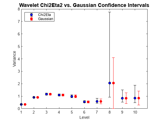
Specify non-default confidence methods using name-value arguments to compare the width of their confidence levels. Note that for Gaussian confidence level intervals, it is possible to obtain negative lower confidence bounds.

Obtain the MODWT of the Southern Oscillation Index data using the Fejér-Korovkin wavelet with eight coefficients.

load soi
wsoi = modwt(soi,"fk8");

Use the Chi2Eta and Gaussian confidence methods to obtain the variances and confidence interval bounds for each method.

[wvar_c,wvarci_c] = modwtvar(wsoi,"fk8",[],ConfidenceMethod="chi2eta1");
[wvar_g,wvarci_g] = modwtvar(wsoi,"fk8",[],ConfidenceMethod="gaussian");

Compute the upper and lower errors for each confidence interval and plot the results. Note that the Gaussian intervals are slightly shifted to enable better visualization.

errlower_c = wvar_c-wvarci_c(:,1);
errupper_c = wvarci_c(:,2)-wvar_c;

errlower_g = wvar_g(:,1)-wvarci_g(:,1);
errupper_g = wvarci_g(:,2)-wvar_g;

errorbar(1:10,wvar_c(1:10),errlower_c(1:10),...
    errupper_c(1:10),"ko",markerfacecolor="b")
hold on
xoffset = (1.3:10.3);
errorbar(xoffset,wvar_g(1:10),errlower_g(1:10),...
    errupper_g(1:10),"ro",markerfacecolor="r")

title("Wavelet Chi2Eta2 vs. Gaussian Confidence Intervals",fontsize=14)
ylabel("Variance")
xlabel("Level")
ax = gca;
ax.XTick = [1:10];
legend("Chi2Eta","Gaussian",Location="northwest")
hold off

Figure contains an axes object. The axes object with title Wavelet Chi2Eta2 vs. Gaussian Confidence Intervals, xlabel Level, ylabel Variance contains 2 objects of type errorbar. These objects represent Chi2Eta, Gaussian.

Compare Number of Coefficients for Unbiased and Biased Variance Estimates

Open Live Script

Compare the number of coefficients for unbiased and biased wavelet variance estimates. For the unbiased (default) estimates, the number of nonboundary coefficients decreases by scale. For biased estimates, the number of coefficients matches the number of input rows and is constant for every scale.

Obtain the MODWT of the Southern Oscillation Index data using the Fejér-Korovkin wavelet with eight coefficients.

load soi
wsoi = modwt(soi,"fk8");

Compute the unbiased and biased estimates of the wavelet variance down to level ten. The number of coefficients used in the unbiased estimates decrease by scale.

[wvar_unb,wvarci_unb,nj_unb] = modwtvar(wsoi,"fk8");
[wvar_b,wvarci_b,nj_b] = modwtvar(wsoi,"fk8",[],EstimatorType="biased");
[nj_unb(1:10),nj_b(1:10)]

ans = 10×2

       12991       12998
       12977       12998
       12949       12998
       12893       12998
       12781       12998
       12557       12998
       12109       12998
       11213       12998
        9421       12998
        5837       12998

Table of Wavelet Variance Estimates Using Gaussian Confidence Intervals

Open Live Script

Compute the MODWT of the Southern Oscillation Index data using the Fejér- Korovkin wavelet with eight coefficients.

load soi
wsoi = modwt(soi,"fk8");

Compute a variance table for the data. The table contains the number of nonboundary coefficients, the lower and upper confidence level bounds, and the variance estimate for each level.

[wvartable] = modwtvar(wsoi,"fk8",0.90,"table", ...
    ConfidenceMethod="gaussian")

wvartable=10×4 table
            NJ       Lower     Variance     Upper 
           _____    _______    ________    _______

    D1     12991     0.3291    0.33848     0.34786
    D2     12977    0.87172     0.9034     0.93508
    D3     12949     1.1041     1.1628      1.2216
    D4     12893     1.0204     1.0933      1.1662
    D5     12781     0.8833    0.98255      1.0818
    D6     12557    0.47178    0.54152     0.61125
    D7     12109    0.41916    0.57934     0.73951
    D8     11213    0.33639      2.055      3.7736
    D9      9421     0.4752    0.83369      1.1922
    D10     5837    0.37485    0.84386      1.3129

Input Arguments

collapse all

`w` — MODWT transform matrix
matrix

MODWT transform, specified as a matrix. w is the output of modwt.

Data Types: double

`wname` — Wavelet
`"sym4"` (default) | character vector | string scalar | positive even scalar

Wavelet, specified as a character vector or string scalar corresponding to a valid wavelet, or as a positive even scalar indicating the length of the wavelet and scaling filters. The wavelet filter length must match the length used in the MODWT of the input.

If you use Name,Value arguments or the "table" syntax and you do not specify a wname , you must use [] as the second argument.

`conflevel` — Confidence level
0.95 (default) | real scalar greater than 0 and less than 1

Confidence level, specified as a real scalar value greater than 0 and less than 1. The confidence level determines the coverage probability of the confidence intervals. If you specify "table" as an input, the confidence levels are also shown in wvartable.

Name-Value Arguments

Specify optional pairs of arguments as Name1=Value1,...,NameN=ValueN, where Name is the argument name and Value is the corresponding value. Name-value arguments must appear after other arguments, but the order of the pairs does not matter.

Example: ConfidenceMethod="gaussian" specifies the Gaussian method used to compute the confidence intervals.

Before R2021a, use commas to separate each name and value, and enclose Name in quotes.

Example: 'EstimatorType','biased' specifies a biased estimator.

`EstimatorType` — Estimator
`"unbiased"` (default) | `"biased"`

Type of estimator used for variance estimates and confidence bounds, specified as one of these values.

"unbiased" — Unbiased estimator, which identifies and removes boundary coefficients prior to computing the variance estimates and confidence bounds. Unbiased estimates are used more frequently for wavelet variance computations.
"biased" — Biased estimator, which uses all coefficients to compute the variance estimates and confidence bounds.

`ConfidenceMethod` — Confidence method
`"chi2eta3"` (default) | `"chi2eta1"` | `"gaussian"`

Confidence method used to compute the confidence intervals, specified as one of these values:

`"chi2eta3"`	Chi-square probability density method three, which determines the degrees of freedom.[1].
`"chi2eta1"`	Chi-square probability density method one, which determines the degrees of freedom [1].
`"gaussian"`	Gaussian method [1]. This method can result in negative lower bounds.

See Algorithm for information on each of these confidence methods.

`Boundary` — Boundary condition
`"periodic"` (default) | `"reflection"`

Boundary condition used to compute the variance estimates and confidence bounds, specified as one of these values:

"periodic" Periodic boundary handling, which does not change the original signal before computing the MODWT. If modwt uses periodic boundary handling, you must specify Boundary="periodic" for modwtvar to obtain a correct estimate.

"reflection" Reflection boundary handling. If the MODWT uses reflection boundary handling, you must also specify Boundary="reflection" for modwtvar to obtain a correct unbiased estimate. The MODWT, with reflection boundary handling, extends the original signal symmetrically at the right boundary to twice the signal length. The MODWTVAR algorithm has to know about this extended signal to calculate the correct unbiased estimate.
For biased estimators, all the coefficients are used to form the variance estimates and confidence intervals regardless of the boundary handling.

Output Arguments

collapse all

`wvar` — Wavelet variance estimates
matrix

Wavelet variance estimates, returned as vector. The number of elements in wvar depends on the number of scales in the input matrix and, for unbiased estimates, on the wavelet length. For the unbiased case, modwtvar returns estimates only where nonboundary coefficients exist. This condition is satisfied when the transform level is not greater than floor(log2(N/(L-1)+1)), where N is the input signal length and L is the length of the wavelet filter. The number of biased estimates equals the input signal length. If the final level has sufficient nonboundary coefficients, modwtvar returns the scaling variance in the final element of wvar.

`wvarci` — Confidence intervals for each variance estimate
matrix

Confidence bounds, expressed as upper and lower confidence bounds, for the variance estimates in wvar, returned as a matrix. The default is 95% confidence bounds, but you can use a different value using the conflevel input argument. The confidence bounds matrix is M-by-2, where M is the number of levels. For unbiased estimates, the number of levels is limited by the number of nonboundary coefficients. For biased estimates, all levels are used. The first column of the confidence interval matrix contains the lower confidence bound and the second column contains the upper confidence bound. By default, modwtvar calculates the confidence intervals using the chi-square probability density, with the equivalent degrees of freedom estimated using the "Chi2Eta3" confidence method.

`nj` — Number of coefficients by level
vector

Number of nonboundary coefficients by scale, returned as a vector. For unbiased estimates, nj is the number of nonboundary coefficients and decreases by level. For biased estimates, nj is a vector of constants equal to the number of columns in the input matrix.

`wvartable` — Variance table
table

Variance table, returned as a MATLAB table. The four variables in the table are:

NJ — Number of MODWT coefficients by level. For biased estimates, NJ is the number of coefficients in the MODWT. For unbiased estimates, NJ is the number of nonboundary coefficients.
Lower — Lower confidence bound for the variance estimate.
Variance — Variance estimate by level.
Upper — Upper confidence bound for the variance estimate.

The row names of wvartable indicate the type and level of each estimate. For example, D1 indicates that the row corresponds to a wavelet or detail estimate at level 1. S6 indicates that the row corresponds to the scaling estimate at level 6. The scaling variance is computed for the final level of the MODWT. For unbiased estimates, modwtvar computes the scaling variance only when nonboundary scaling coefficients exist.

Algorithms

The following expressions define the variance and confidence methods used in the MODWTVAR. The variables are:

N_j — Number of coefficients at level j
v² — Variance
j — Level
W_j,t — Wavelet coefficients

The variance estimate is

${\hat{v}}_{j}^{2} = \frac{1}{N_{j}} \sum_{t = 0}^{N_{j} - 1} W_{j, t}^{2}$

The degrees of freedom for the Chi2Eta1 (chi2eta1) method are defined as

$η_{1} = \frac{N_{j} {\hat{v}}_{j}^{4}}{{\hat{A}}_{j}}$

where

${\hat{A}}_{j} = \frac{1}{2} {\int_{- 1 / 2}^{1 / 2} [{\hat{S}}_{j}^{(p)} (f)]}^{2} d f .$

In this equation, ${\hat{S}}_{j}^{(p)}$ is the spectral density function estimate of the wavelet coefficients at level j.

The chi-square statistic is

$\frac{η_{1} N_{j} {\hat{v}}_{j}^{2}}{v_{j}^{2}} ~ Χ_{η_{1}}^{2}$

The degrees of freedom for the Chi2Eta3 (chi2eta3) method are defined as

$η_{3} = max (\frac{N_{j}}{2^{j}}, 1)$

The chi-square statistic is

$\frac{η_{3} N_{j} {\hat{v}}_{j}^{2}}{v_{j}^{2}} ~ Χ_{η_{3}}^{2}$

For the Gaussian method, the statistic

$\frac{N_{j}^{1 / 2} (({\hat{v}}_{j}^{2} - v_{j}^{2}))}{{(2 {\hat{A}}_{j})}^{1 / 2}}$

is distributed as N(0,1). The variable ${\hat{A}}_{j}$ is as described for chi2eta1.

References

[1] Percival, Donald B., and Andrew T. Walden. Wavelet Methods for Time Series Analysis. Cambridge: Cambridge University Press, 2000.

[2] Percival, Donald B., and Debashis Mondal. “22 - A Wavelet Variance Primer.” In Time Series Analysis: Methods and Applications, edited by Tata Subba Rao, Suhasini Subba Rao, and C. Radhakrishna Rao, 1st ed., 623–57. Handbook of Statistics, v. 30. Amsterdam ; London: Elsevier, 2012. https://doi.org/10.1016/B978-0-444-53858-1.00022-3.

[3] Cornish, Charles R., Christopher S. Bretherton, and Donald B. Percival. “Maximal Overlap Wavelet Statistical Analysis With Application to Atmospheric Turbulence.” Boundary-Layer Meteorology 119, no. 2 (May 2006): 339–74. https://doi.org/10.1007/s10546-005-9011-y.

Extended Capabilities

C/C++ Code Generation
Generate C and C++ code using MATLAB® Coder™.

Usage notes and limitations:

The input wname must be constant.
The input conflevel must be defined as a scalar.
Plotting is not supported.

Version History

Introduced in R2015b

modwtvar

Syntax

Description

Examples

Wavelet Variance Using Default Wavelet

Wavelet Variance Using Specified Wavelet

Variance Estimates and Confidence Intervals Using MODWTVAR

Wavelet Confidence Intervals

Compare Chi2Eta2 and Gaussian Confidence Intervals

Compare Number of Coefficients for Unbiased and Biased Variance Estimates

Table of Wavelet Variance Estimates Using Gaussian Confidence Intervals

Input Arguments

`w` — MODWT transform matrix
matrix

`wname` — Wavelet
`"sym4"` (default) | character vector | string scalar | positive even scalar

`conflevel` — Confidence level
0.95 (default) | real scalar greater than 0 and less than 1

Name-Value Arguments

`EstimatorType` — Estimator
`"unbiased"` (default) | `"biased"`

`ConfidenceMethod` — Confidence method
`"chi2eta3"` (default) | `"chi2eta1"` | `"gaussian"`

`Boundary` — Boundary condition
`"periodic"` (default) | `"reflection"`

Output Arguments

`wvar` — Wavelet variance estimates
matrix

`wvarci` — Confidence intervals for each variance estimate
matrix

`nj` — Number of coefficients by level
vector

`wvartable` — Variance table
table

Algorithms

References

Extended Capabilities

C/C++ Code Generation
Generate C and C++ code using MATLAB® Coder™.

Version History

See Also

Apps

Functions

Topics

modwtvar

Syntax

Description

Examples

Wavelet Variance Using Default Wavelet

Wavelet Variance Using Specified Wavelet

Variance Estimates and Confidence Intervals Using MODWTVAR

Wavelet Confidence Intervals

Compare Chi2Eta2 and Gaussian Confidence Intervals

Compare Number of Coefficients for Unbiased and Biased Variance Estimates

Table of Wavelet Variance Estimates Using Gaussian Confidence Intervals

Input Arguments

w — MODWT transform matrix matrix

wname — Wavelet "sym4" (default) | character vector | string scalar | positive even scalar

conflevel — Confidence level 0.95 (default) | real scalar greater than 0 and less than 1

Name-Value Arguments

EstimatorType — Estimator "unbiased" (default) | "biased"

ConfidenceMethod — Confidence method "chi2eta3" (default) | "chi2eta1" | "gaussian"

Boundary — Boundary condition "periodic" (default) | "reflection"

Output Arguments

wvar — Wavelet variance estimates matrix

wvarci — Confidence intervals for each variance estimate matrix

nj — Number of coefficients by level vector

wvartable — Variance table table

Algorithms

References

Extended Capabilities

C/C++ Code Generation Generate C and C++ code using MATLAB® Coder™.

Version History

See Also

Apps

Functions

Topics

`w` — MODWT transform matrix
matrix

`wname` — Wavelet
`"sym4"` (default) | character vector | string scalar | positive even scalar

`conflevel` — Confidence level
0.95 (default) | real scalar greater than 0 and less than 1

`EstimatorType` — Estimator
`"unbiased"` (default) | `"biased"`

`ConfidenceMethod` — Confidence method
`"chi2eta3"` (default) | `"chi2eta1"` | `"gaussian"`

`Boundary` — Boundary condition
`"periodic"` (default) | `"reflection"`

`wvar` — Wavelet variance estimates
matrix

`wvarci` — Confidence intervals for each variance estimate
matrix

`nj` — Number of coefficients by level
vector

`wvartable` — Variance table
table

C/C++ Code Generation
Generate C and C++ code using MATLAB® Coder™.