Comparing MODWT and MODWTMRA

Open Live Script

This example demonstrates the differences between the MODWT and MODWTMRA. The MODWT partitions a signal's energy across detail coefficients and scaling coefficients. The MODWTMRA projects a signal onto wavelet subspaces and a scaling subspace.

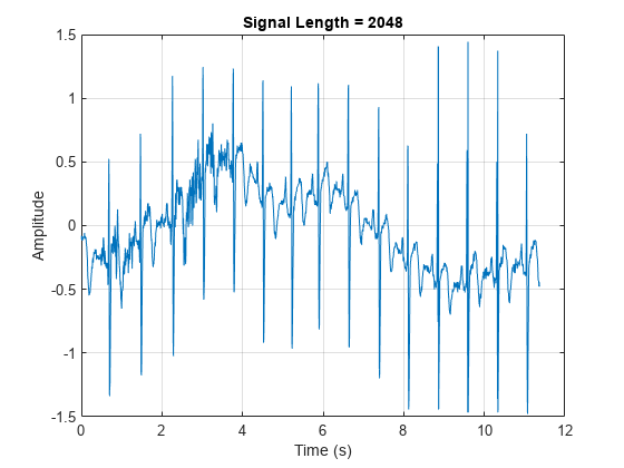
Choose the sym6 wavelet. Load and plot an electrocardiogram (ECG) signal. The sampling frequency for the ECG signal is 180 hertz. The data are taken from Percival and Walden (2000), p.125 (data originally provided by William Constantine and Per Reinhall, University of Washington).

load wecg
t = (0:numel(wecg)-1)/180;
wv = 'sym6';
plot(t,wecg)
grid on
title(['Signal Length = ',num2str(numel(wecg))])
xlabel('Time (s)')
ylabel('Amplitude')

Take the MODWT of the signal.

wtecg = modwt(wecg,wv);

The input data are samples of a function $f (x)$ evaluated at $N$ time points. The function can be expressed as a linear combination of the scaling function $ϕ (x)$ and wavelet $ψ (x)$ at varying scales and translations: $f (x) = \sum_{k = 0}^{N - 1} c_{k} 2^{- J_{0} / 2} ϕ (2^{- J_{0}} x - k) + \sum_{j = 1}^{J_{0}} f_{j} (x)$ , where $f_{j} (x) = \sum_{k = 0}^{N - 1} d_{j, k} 2^{- j / 2} ψ (2^{- j} x - k)$ and $J_{0}$ is the number of levels of wavelet decomposition. The first sum is the coarse scale approximation of the signal, and the $f_{j} (x)$ are the details at successive scales. MODWT returns the $N$ coefficients ${c_{k}}$ and the $(J_{0} \times N)$ detail coefficients ${d_{j, k}}$ of the expansion. Each row in wtecg contains the coefficients at a different scale.

When taking the MODWT of a signal of length $N$ , there are $floor (\log_{2} (N))$ levels of decomposition by default. Detail coefficients are produced at each level. Scaling coefficients are returned only for the final level. In this example, $N = 2048$ , $J_{0} = floor (\log 2 (2048)) = 11$ , and the number of rows in wtecg is $J_{0} + 1 = 11 + 1 = 12$ .

The MODWT partitions the energy across the various scales and scaling coefficients: ${| | X | |}^{2} = \sum_{j = 1}^{J_{0}} {| | W_{j} | |}^{2} + {| | V_{J_{0}} | |}^{2}$ , where $X$ is the input data, $W_{j}$ are the detail coefficients at scale $j$ , and $V_{J_{0}}$ are the final-level scaling coefficients.

Compute the energy at each scale, and evaluate their sum.

energy_by_scales = sum(wtecg.^2,2);
Levels = {'D1';'D2';'D3';'D4';'D5';'D6';...
    'D7';'D8';'D9';'D10';'D11';'A11'};
energy_table = table(Levels,energy_by_scales);
disp(energy_table)

    Levels     energy_by_scales
    _______    ________________

    {'D1' }         14.063     
    {'D2' }         20.612     
    {'D3' }         37.716     
    {'D4' }         25.123     
    {'D5' }         17.437     
    {'D6' }         8.9852     
    {'D7' }         1.2906     
    {'D8' }         4.7278     
    {'D9' }         12.205     
    {'D10'}         76.428     
    {'D11'}         76.268     
    {'A11'}         3.4192

energy_total = varfun(@sum,energy_table(:,2))

energy_total=table
    sum_energy_by_scales
    ____________________

           298.28

Confirm the MODWT is energy-preserving by computing the energy of the signal and comparing it with the sum of the energies over all scales.

energy_ecg = sum(wecg.^2);
max(abs(energy_total.sum_energy_by_scales-energy_ecg))

ans = 7.4402e-10

Take the MODWTMRA of the signal.

mraecg = modwtmra(wtecg,wv);

MODWTMRA returns the projections of the function $f (x)$ onto the various wavelet subspaces and final scaling space. That is, MODWTMRA returns $\sum_{k = 0}^{N - 1} c_{k} 2^{- J_{0} / 2} ϕ (2^{- J_{0}} x - k)$ and the $J_{0}$ -many ${f_{j} (x)}$ evaluated at $N$ time points. Each row in mraecg is a projection of $f (x)$ onto a different subspace. This means the original signal can be recovered by adding all the projections. This is not true in the case of the MODWT. Adding the coefficients in wtecg will not recover the original signal.

Choose a time point, add the projections of $f (x)$ evaluated at that time point, and compare with the original signal.

time_point = 1000;
abs(sum(mraecg(:,time_point))-wecg(time_point))

ans = 3.0846e-13

Confirm that, unlike MODWT, MODWTMRA is not an energy-preserving transform.

energy_ecg = sum(wecg.^2);
energy_mra_scales = sum(mraecg.^2,2);
energy_mra = sum(energy_mra_scales);
max(abs(energy_mra-energy_ecg))

ans = 115.7053

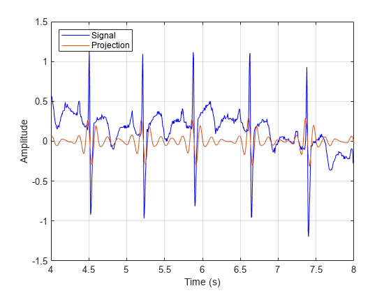
The MODWTMRA is a zero-phase filtering of the signal. Features will be time-aligned. Show this by plotting the original signal and one of its projections. To better illustrate the alignment, zoom in.

plot(t,wecg,'b')
hold on
plot(t,mraecg(4,:),'-')
hold off
grid on
xlim([4 8])
legend('Signal','Projection','Location','northwest')
xlabel('Time (s)')
ylabel('Amplitude')

Make a similar plot using the MODWT coefficients at the same scale. Features will not be time-aligned. The MODWT is not a zero-phase filtering of the input.

plot(t,wecg,'b')
hold on
plot(t,wtecg(4,:),'-')
hold off
grid on
xlim([4 8])
legend('Signal','Coefficients','Location','northwest')
xlabel('Time (s)')
ylabel('Amplitude')

References

[1] Percival, D. B., and A. T. Walden. Wavelet Methods for Time Series Analysis. Cambridge, UK: Cambridge University Press, 2000.