Frequency- and Time-Localized Reconstruction from the Continuous Wavelet Transform

Reconstruct a frequency-localized approximation of the Kobe earthquake data. The data is sampled at 1 Hz. Extract information from the CWT for frequencies in the range of [0.030, 0.070] Hz.

load kobe
Fs = 1;

Obtain the CWT of the data.

[wt,f] = cwt(kobe,Fs);

Reconstruct the earthquake data, adding the signal mean back into the transformed data.

xrec = icwt(wt,[],f,[0.030 0.070],SignalMean=mean(kobe));

Plot and compare the original data and the data for frequencies in the range of [0.030, 0.070] Hz.

t = (0:numel(kobe)-1)/60;
tiledlayout(2,1)
nexttile
plot(t,kobe)
grid on
title("Original Data")
nexttile
plot(t,xrec)
grid on
xlabel("Time (mins)")
title("Bandpass Filtered Reconstruction [0.030 0.070] Hz")

You can also use time periods, instead of frequency, with the CWT. Load the El Nino data, which is sampled monthly. Obtain its CWT, specifying the time period in years.

load ninoairdata
[cfs,period] = cwt(nino,years(1/12));

Obtain the inverse CWT for years 2 through 8.

xrec = icwt(cfs,[],period,[years(2) years(8)]);

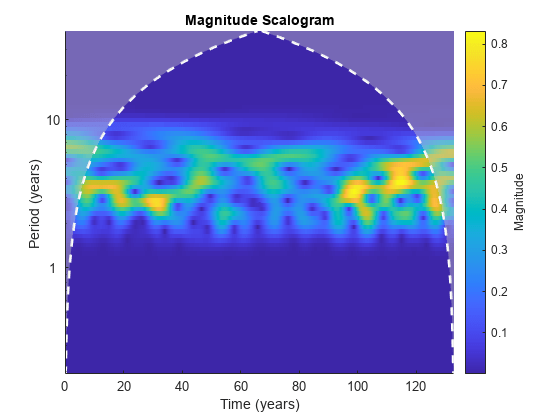
Plot the CWT of the reconstructed data. Note the absence of energy outside the band of periods from 2 to 8 years.

figure
cwt(xrec,years(1/12))

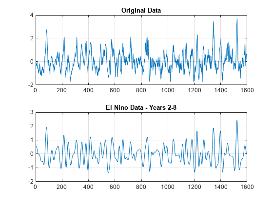
Compare the original data with the reconstructed data for years 2 through 8.

figure
tiledlayout(2,1)
nexttile
plot(datayear,nino)
grid on
title("Original Data")
nexttile
plot(datayear,xrec)
grid on
title("El Nino Data - Years 2-8")

See Also

Apps

• Wavelet Time-Frequency Analyzer

Objects

• cwtfilterbank

Functions

• cwt | icwt

Related Topics

• Practical Introduction to Time-Frequency Analysis Using the Continuous Wavelet Transform