Sample Rate Conversion for an LTE Receiver

Introduction

The LTE HDL Cell Search, LTE HDL MIB Recovery, and LTE HDL SIB1 Recovery reference applications require an input sampling rate of 30.72 Msps. In practice, the sampling rate presented to hardware may differ from this, for example due to choice of components or system design decisions. Therefore, sample rate conversion may be required to integrate these reference applications into a larger system. The model shown in this example converts from 125, 140, or 150 Msps to 30.72 Msps using two FIR Decimation filters and a programmable Farrow rate converter. The rate changes from 125, 140 or 150 Msps to 30.72 Msps were deliberately chosen because they are not trivial to implement yet represent an example of the type of rate change often required in a radio receiver.

Sample Rate Converter Design Overview

At the top level, you can program the rate converter using the FarrowSelect input. This allows you to select between three predefined input sampling rates - 125, 140 or 150 Msps. You can program the Farrow Rate Converter to have any rate change in practice. The default rates are just chosen as an example. The default conversion from 150 Msps to 30.72 Msps corresponds to a rate change factor of 0.2048. This is implemented with the filter chain shown. First, a Farrow rate converter is used to make a fine adjustment to the sample rate by a factor of 150/30.72*4 = 1.2207. Next, the signal is decimated by two (i.e. a rate change of 1/2) using a halfband filter. Last, a decimating FIR filter implements the final decimate-by-two stage.

Choice of Filters

The reasons for using this set of filters are as follows:

Clock Rate and Valid Signals

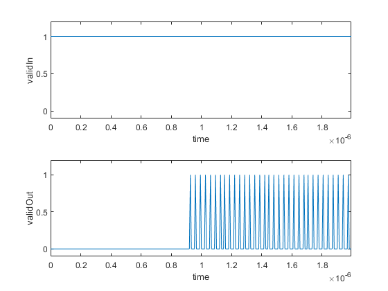
In this example, the default clock rate is 150 MHz and the default input sampling rate is 150 Msps. Sampling rates are conveyed by the duty cycle of the valid signals (the percentage of time that valid is true) at each stage. For example, the duty cycle of validIn is 100% and the duty cycle of farrowValidOut is 81.92% and has an irregular, non-periodic pattern. It follows the true, false, true, false ... pattern most of the time, however it will occasionally miss a true cycle to represent the rate correctly. The FIR Decimator halves the sampling rate again, however it also has an irregular, non-periodic valid output pattern because it is driven by the Farrow Rate Converter. validOut has a duty cycle of 20.48%.

While the simulation shown in this example uses a validIn duty cycle of 100%, the sample rate converter can accept any valid input pattern with any duty cycle. This is useful in scenarios where the hardware clock rate is greater than the input sampling rate.

Top Level Parameters

Configure the top level parameters of the sample rate converter. FsADC is the input rate, while FsLTERx is the output rate; that is, the input to the LTE receiver. You can modify FsADC to be 100e6, 125e6, or 150e6, so long as you drive the FarrowSelect switch with the correct value. Fpass is the passband cut-off frequency and is set to 10 MHz to accommodate the maximum possible LTE bandwidth of 20 MHz. Fstop is set to the Nyquist rate, however can be adjusted if more out-of-band signal rejection is required. Ast is the stopband attenuation in dBs, and Ap is the desired amount of passband ripple.

FsADC   = 150e6;
FsLTERx = 30.72e6;
Fpass   = 10e6;
Fstop   = FsLTERx/2;
Ast     = 60;
Ap      = 0.1;

Farrow Rate Converter

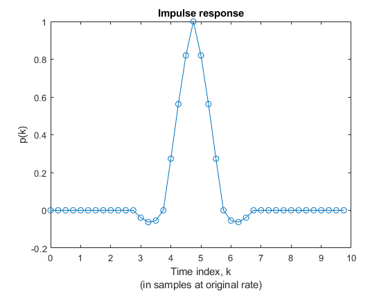
In this example, the Farrow Rate Converter uses the default 3rd order LaGrange coefficients. These are derived from a closed form solution and in general work for any rate change. The Farrow filter structure is the same as that used in the dsp.VariableIntegerDelay and dsp.FarrowRateConverter System objects.

Define the key parameters of the Farrow rate converter. FsIn and FsOut are the input and output rates respectively.

farrow.FsIn    = FsADC;
farrow.FsOut   = 4*FsLTERx;

Now, we can evaluate the Farrow Rate Converter.

% Generate an impulse input with a length of Lx samples.
Lx = 10;
x = zeros(Lx,1);
x(1) = 1;

% Evaluate the oversampled impulse response of the
% Farrow-based Variable Fractional Delay.
% Instantiate a variable fractional delay object.
% Pass the impulse through it at N different fractional
% delays from 0 to 1-(1/N) in steps of 1/N and store
% the results in the oversampled response vector p.

vfd = dsp.VariableFractionalDelay( ...
    'InterpolationMethod','Farrow');

N = 4;
Lp = N * Lx;
p = zeros(Lp,1);


for n=1:N
    p(n:N:end) = vfd(x,4+(N-n)/N);
end

% Plot the impulse response
figure(1); clf;
t = (0:length(p)-1)/N;
plot(t,p,'-o');
title("Impulse response");
xlabel("Time index, k" + newline + "(in samples at original rate)");
ylabel("p(k)");
print ImpulseResponse.png -dpng

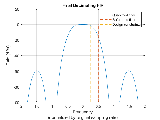
% Plot the magnitude response
figure(2); clf;
Lfft = 1024;
Pmag = 20*log(abs(fft(p/N,1024)));
f = (0:Lfft-1) * N / Lfft;
plot(f-N/2,fftshift(Pmag)); hold on;
ax = axis;
plot([1/2 1/2],[ax(3) ax(4)],'--');
plot([1/4 1/4],[ax(3) ax(4)],'--');
plot([1/8 1/8],[ax(3) ax(4)],'--');
axis([ax(1) ax(2) -100 20]);
grid on;
title("Magnitude");
xlabel("Frequency" + newline + "(normalized by original sampling rate)");
ylabel("Gain (dBs)");
legend("Filter response","Fs/2","Fs/4","Fs/8");
print MagnitudeResponse.png -dpng

Decimating FIR Filters

Design the intermediate and final FIR filter stages. Both filters use 16-bit coefficients. For convenience, the coefficients data type is defined.

FIRCoeffsDT = numerictype(1,16,15);

Halfband Decimator

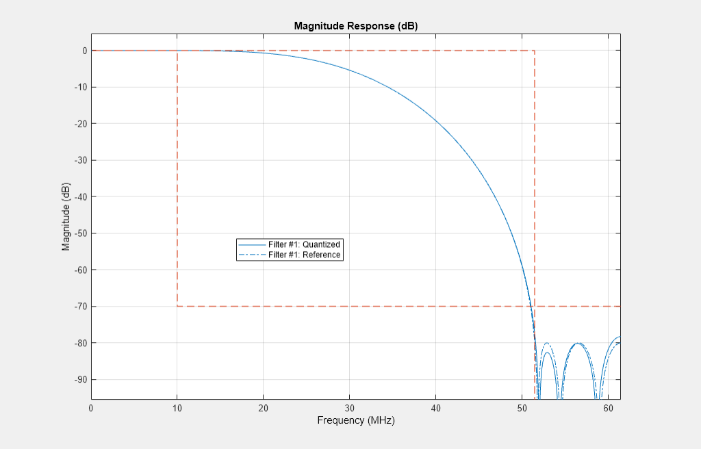
Design a halfband filter to efficiently decimate the input by 2.

hbParams.FsIn                = farrow.FsOut;
hbParams.FsOut               = farrow.FsOut/2;
hbParams.TransitionWidth     = hbParams.FsOut - 2*Fpass;
hbParams.StopbandAttenuation = Ast + 10;

hbSpec = fdesign.decimator(2,'halfband',...
    'Tw,Ast',...
    hbParams.TransitionWidth, ...
    hbParams.StopbandAttenuation,...
    hbParams.FsIn);

halfband = design(hbSpec,'SystemObject',true);

halfband.FullPrecisionOverride = false;
halfband.CoefficientsDataType  = 'Custom';
halfband.CustomCoefficientsDataType = numerictype([],...
    FIRCoeffsDT.WordLength,FIRCoeffsDT.FractionLength);

Plot the frequency response of the filter, including the quantized response.

filterAnalyzer(halfband,'arithmetic','fixed');
SRCTestUtils.setPlotNameAndTitle('Halfband FIR');
legend('Quantized filter','Reference filter','Design constraints');

Final FIR Decimator

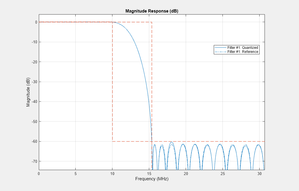
Design the final decimate-by-2 FIR filtering stage.

finalSpec = fdesign.decimator(2,'lowpass',...
    'Fp,Fst,Ap,Ast',Fpass,Fstop,Ap,Ast,hbParams.FsOut);

finalFilt = design(finalSpec,'equiripple','SystemObject',true);

finalFilt.FullPrecisionOverride = false;
finalFilt.CoefficientsDataType  = 'Custom';
finalFilt.CustomCoefficientsDataType = numerictype([],...
    FIRCoeffsDT.WordLength,FIRCoeffsDT.FractionLength);

Plot the frequency response of the filter, including the quantized response.

filterAnalyzer(finalFilt,'arithmetic','fixed');
SRCTestUtils.setPlotNameAndTitle('Final Decimating FIR');
legend('Quantized filter','Reference filter','Design constraints');

Simulink HDL Implementation

Open the model and update the diagram. The top level of the model is shown. HDL code can be generated for the Sample Rate Converter subsystem.

stopTime  = 0;
dataIn    = 0;
validIn   = false;
modelName = 'SampleRateConversionHDL';
open_system(modelName);
set_param(modelName,'SimulationCommand','Update');
set_param(modelName, 'Open','on');

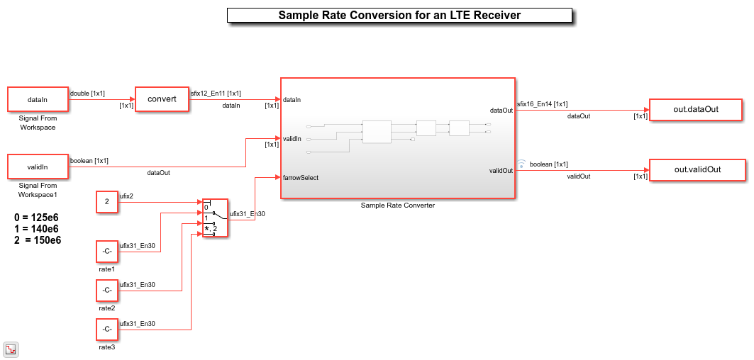
As discussed, the sample rate converter contains a Farrow rate converter, a halfband filter, and a final FIR decimation stage. The Farrow has a ready signal, which is not used in decimation and therefore is terminated. When the overall rate change corresponds to interpolation, the ready is useful for pacing the input. The two FIR Decimator blocks are configured to use the coefficients previously designed and stored in FIR System objects. As mentioned previously, the final FIR Decimator can use resource sharing, seeing as the input is only valid one every 2 cycles. This is configured by setting "Minimum number of cycles between valid input" to 2.

set_param([modelName '/Sample Rate Converter'],'Open','on');

Validation and Verification

An LTE test signal is generated at 150 Msps and passed through the rate converter. An Error Vector Magnitude (EVM) measurement is then performed, confirming that the resampler is suitable for use in an LTE receiver. For reference, three different methods are used to resample the signal to 30.72 Msps and their EVM results compared. The three methods are:

In addition, to confirm correct operation of the HDL implementation, the root-mean-square error between the outputs of the MATLAB and Simulink rate converter models is computed.

Generate a 20 MHz LTE test signal sampled at 150 Msps.

rng(0);
enb              = lteRMCDL('R.9');
enb.TotSubframes = 2;
[tx, ~, sigInfo] = lteRMCDLTool(enb,randi([0 1],1000,1));
dataIn = resample(tx,FsADC,sigInfo.SamplingRate);
dataIn  = 0.95 * dataIn / max(abs(dataIn));
validIn = true(size(dataIn));

Use the resample function to resample the received signal from the ADC rate to 30.72 Msps. This provides a good quality reference to compare to the rate converter.

resampleOut = resample(dataIn,FsLTERx,FsADC);

Pass the signal through a MATLAB model of the rate converter.

farrowFilt        = dsp.FarrowRateConverter(farrow.FsIn,farrow.FsOut);
farrowOut         = farrowFilt(dataIn);
halfbandOut       = halfband(farrowOut);
floatResamplerOut = finalFilt(halfbandOut);

Pass the signal through the fixed-point Simulink HDL implementation model.

stopTime       = (length(dataIn)+1000)/FsADC;
simOut         = sim(modelName);
fiResamplerOut = simOut.dataOut(simOut.validOut);
fiResamplerOut = fiResamplerOut(1:length(floatResamplerOut));

Plot validIn and validOut to show the overall rate change of the sample rate converter. validIn is always HIGH, whereas validOut is HIGH about a quarter (0.24576%) of the time.

srcPlots.validSignals = figure;
Ns = 300;
validInSlice = validIn(1:Ns);
validOutSlice = simOut.validOut(1:Ns);
subplot(2,1,1);
plot((0:Ns-1)/FsADC,validInSlice);
axis([0 (Ns-1)/FsADC -0.1 1.2]);
ylabel('validIn');
xlabel('time');
subplot(2,1,2);
plot((0:Ns-1)/FsADC,validOutSlice);
axis([0 (Ns-1)/FsADC -0.1 1.2]);
ylabel('validOut');
xlabel('time');

Compute the root mean square error between the outputs of the MATLAB and Simulink models of the rate converter

e = floatResamplerOut-fiResamplerOut;
rootMeanSquareError = sqrt((e' * e)/length(e));
disp(['Root-mean-square error: ' num2str(rootMeanSquareError)]);

Root-mean-square error: 0.26432

Measure the EVM of all three resampling methods.

results.resampleEVM                    = SRCTestUtils.MeasureEVM(sigInfo,resampleOut,FsLTERx);
results.floatPointSRCEVM               = SRCTestUtils.MeasureEVM(sigInfo,floatResamplerOut,FsLTERx);
[results.fixedPointSRCEVM,fiEqSymbols] = SRCTestUtils.MeasureEVM(sigInfo,fiResamplerOut,FsLTERx);

disp('LTE Error Vector Magnitude (EVM) Measurements');
disp(['     resample function RMS EVM: '  num2str(results.resampleEVM.RMS*100,3) ' %']);
disp(['    resample function Peak EVM: ' num2str(results.resampleEVM.Peak*100,3) ' %']);
disp(['    floating point SRC RMS EVM: '  num2str(results.floatPointSRCEVM.RMS*100,3) ' %']);
disp(['   floating point SRC Peak EVM: ' num2str(results.floatPointSRCEVM.Peak*100,3) ' %']);
disp(['   fixed point HDL SRC RMS EVM: '  num2str(results.fixedPointSRCEVM.RMS*100,3) ' %']);
disp(['  fixed point HDL SRC Peak EVM: ' num2str(results.fixedPointSRCEVM.Peak*100,3) ' %']);

LTE Error Vector Magnitude (EVM) Measurements
     resample function RMS EVM: 0.0138 %
    resample function Peak EVM: 0.0243 %
    floating point SRC RMS EVM: 0.0265 %
   floating point SRC Peak EVM: 0.0645 %
   fixed point HDL SRC RMS EVM: 0.0518 %
  fixed point HDL SRC Peak EVM: 0.246 %

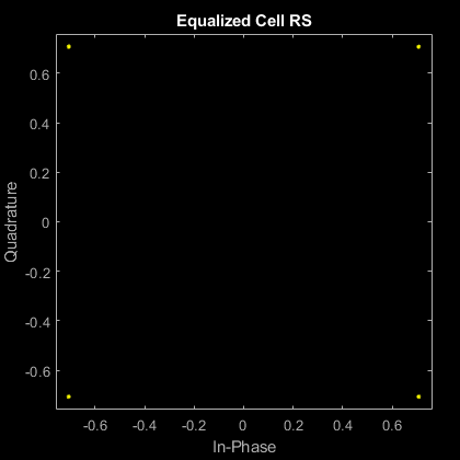
Confirm that the signal quality is high by plotting the equalized pilot symbols from the EVM measurement of the HDL implementation. Note that almost no blurring of the constellation points is visible.

srcPlots.scatterPlot = scatterplot(fiEqSymbols);
SRCTestUtils.setPlotNameAndTitle('Equalized Cell RS');

HDL Code Generation and FPGA Implementation

To generate the HDL code for this example you must have an HDL Coder™ license. Use the makehdl and makehdltb commands to generate HDL code and an HDL testbench for the Sample Rate Converter subsystem. The resulting HDL code was synthesized on a Xilinx® Zynq®-7000 ZC706 evaluation board. The post place and route resource utilization results are shown in the table. The design met timing with a clock frequency of 170 MHz. The critical path is the accumulator in the Farrow Rate Converter. This is implemented in fabric, and has a large wordlength of 32 bits, in order to achieve a high precision rate conversion. To improve timing, either reduce the accumulator wordlength, or map the accumulator to a DSP slice on FPGA.

disp(table(...
    categorical({'LUT'; 'LUTRAM'; 'FF'; 'BRAM'; 'DSP'}),...
    categorical({'1489'; '139'; '7165'; '0'; '64'}),...
    'VariableNames',{'Resource','Usage'}));

    Resource    Usage
    ________    _____

     LUT        1489 
     LUTRAM     139  
     FF         7165 
     BRAM       0    
     DSP        64