Detect Human Presence Using Wireless Sensing with Deep Learning
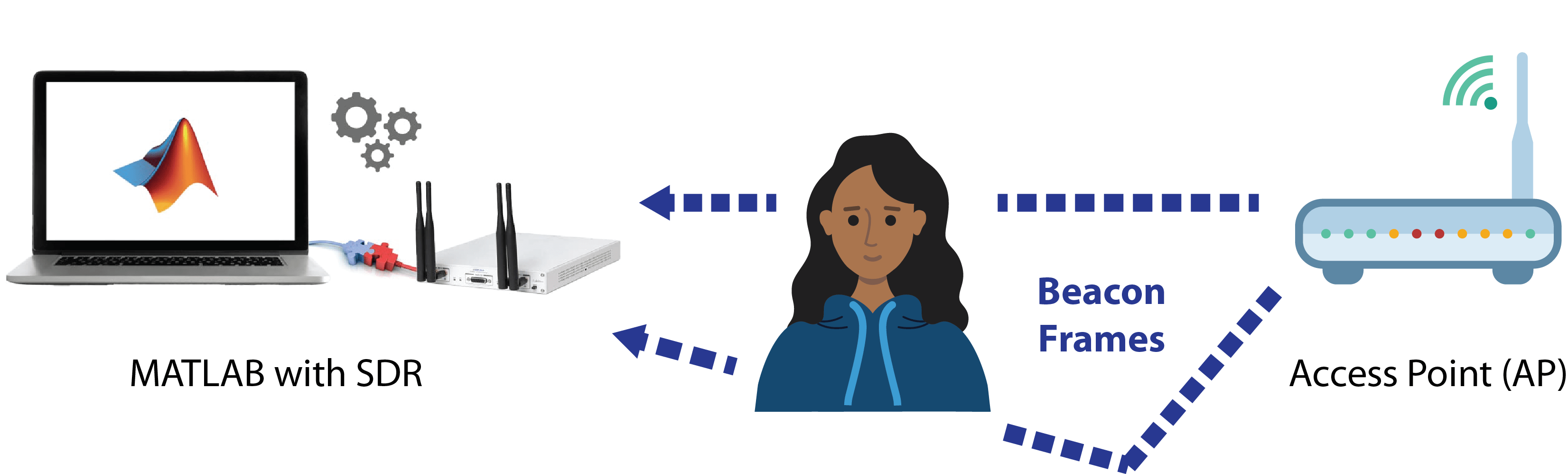
This example shows how to perform wireless sensing to detect human presence using a convolutional neural network (CNN) and the channel state information (CSI) in wireless local area networks. In this example, you can capture beacon frames from real routers with a software defined radio (SDR) to generate your own sensing dataset, or you can use prerecorded data. Then you train a CNN that detects human presence from the live SDR captures or the prerecorded data.
Introduction
Wireless sensing involves utilizing wireless communication technologies to remotely monitor environmental parameters. For example, amplitude and phase changes in the transmitted waveforms can be used to detect the motion of humans, pets, and objects. Advanced signal processing and artificial intelligence/machine learning (AIML) algorithms enable these systems to accurately detect the presence and movements without the need for specialized hardware. Wireless sensing aims to provide several advantages compared to conventional sensor networks, such as non-intrusiveness, wide coverage, low power consumption, accurate tracking, cost-effectiveness, and a privacy-friendly nature.
WLAN sensing (also known as Wi-Fi sensing), uses Wi-Fi networks for high-resolution applications such as emotion, gesture and activity recognition, monitoring vital signs, fall detection, pose estimation, and human presence detection. WLAN sensing is currently being standardized by the IEEE® 802.11bf task group [1]. This technology can sense presence, range, velocity, and location of objects in various environments through subtle changes in the communication channel. CSI is the most common metric for determining the changes in the channel [2]. However, CSI is not typically exposed to you as a user of commercial Wi-Fi devices.
Using WLAN Toolbox™ with a supported SDR, you can capture WLAN waveforms, detect beacon packets, and extract CSI. From this CSI, you create a collection of periodogram images to use as the training and validation datasets for deep learning. Using Deep Learning Toolbox™, you train a CNN and use the trained network for live detection of human presence. Alternatively, you can use the prerecorded dataset to train the CNN and evaluate the presence detection performance against the test dataset. Beacon packets are useful for WLAN sensing as access points (APs) transmit beacon packets periodically. As a result, the sensing resolution is independent of the traffic load at the AP in the temporal domain.
Required Hardware and Software
By default, this example runs using recorded data from a file. For this, you need one of the following:
ADALM-PLUTO (requires Communications Toolbox Support Package for Analog Devices® ADALM-PLUTO Radio). For more information, see ADALM-Pluto Radio.
USRP™ E310/E312 (requires Communications Toolbox Support Package for USRP™ Embedded Series Radio). For more information, see USRP Embedded Series Radio.
200-Series USRP Radio (requires Communications Toolbox Support Package for USRP Radio). For information on how to map an NI™ USRP device to an Ettus Research™ 200-series USRP device, see Supported Hardware and Required Software.
300-Series USRP™ Radio or USRP X410 (requires Wireless Testbench Support Package for NI™ USRP Radios). For more information, see Install Support Package for NI USRP Radios (Wireless Testbench) and Supported Radio Devices (Wireless Testbench).
SDR Setup
This section explains how to set up an SDR for capturing the data that will be used in training and live detection of human presence. If you do not have SDR hardware and plan to use the prerecorded data, you can skip this section.
1) Ensure that you have installed the appropriate support package for the SDR that you intend to use and that you have configured the hardware accordingly.
2) To use your SDR as the data source for training the neural network and then inferencing with the trained CNN, select the useSDR check box.
rxsim.UseSDR =false; % You can skip this section if unchecked
2a) If you are using a radio configured with Wireless Testbench, you have the option to utilize the preamble detector functionality. To do this, select the UsePD check box and calibrate the preamble detector for your environment by tuning the ThresholdGain, ThresholdOffset, and RadioGain parameters. For information on how to calibrate the preamble detector with a WLAN signal, see the OFDM Wi-Fi Scanner Using SDR Preamble Detection example. The USRP N300 and X300 hardware do not support Wireless Testbench preamble detector capabilities.
rxsim.UsePD =false; if rxsim.UseSDR && rxsim.UsePD % Additional preamble detector parameters rxsim.ThresholdGain =
0.23; rxsim.ThresholdOffset =
0.001; end
3) Specify your capture device (rxsim.DeviceName), radio gain (rxsim.RadioGain), and a channel number (rxsim.ChannelNumber) for your operation frequency band (rxsim.FrequencyBand). These settings determine the center frequency from which your SDR captures beacon packets. If you do not know a channel number, use the WLAN Beacon Receiver Using Software-Defined Radio example to determine which channel(s) contain beacon packets.
If you are using an NI USRP hardware with Wireless Testbench, click Update to make your saved radio setup configuration name appear at the top of the dropdown list.
if rxsim.UseSDR deviceNameOptions = hSDRBase.getDeviceNameOptions; % User-defined parameters rxsim.DeviceName =deviceNameOptions(1)
; rxsim.RadioGain =
30; % Can be 'AGC Slow Attack', 'AGC Fast Attack', or an integer value. See relevant documentation for selected radio for valid values of radio gain. rxsim.ChannelNumber =
36; % Valid values for 5 GHz band are integers in range [1, 200] rxsim.FrequencyBand = 5; % in GHz rxsim = setupSDR(rxsim); end
4) Configure these capture parameters:
The number of beacon packets to be extracted from each capture (
rxsim.NumPacketsPerCapture).The number of captures needed to create the dataset and train the neural network (
rxsim.NumCaptures).The beacon interval (
rxsim.BeaconInterval). The default beacon interval for a commercial AP is 100 time units (TUs), where 1 TU equals 1024 microseconds. You typically do not need to adjust the beacon interval value unless you have adjusted the interval of your access point (AP).Filter the beacons based on their SSID if more than one SSID exists on the same channel (
rxsim.BeaconSSID).
if rxsim.UseSDR %#ok<*UNRCH> % User defined parameters rxsim.NumCaptures =10; rxsim.NumPacketsPerCapture =
8; rxsim.BeaconInterval =
100; % in time units (TUs). The default value in typical APs is 100. rxsim.BeaconSSID =
""; % Optional % Calculated parameters rxsim.CaptureDuration = rxsim.BeaconInterval*milliseconds(1.024)*rxsim.NumPacketsPerCapture + milliseconds(5.5); % Add 5.5 ms for beacons located at the end of the waveform % SDR setup is complete msgbox("SDR object configuration is complete! Run steps 1 and 2 to capture data.") return % Stop execution end
System Description
This example uses the following process to obtain CSI images for human presence detection:
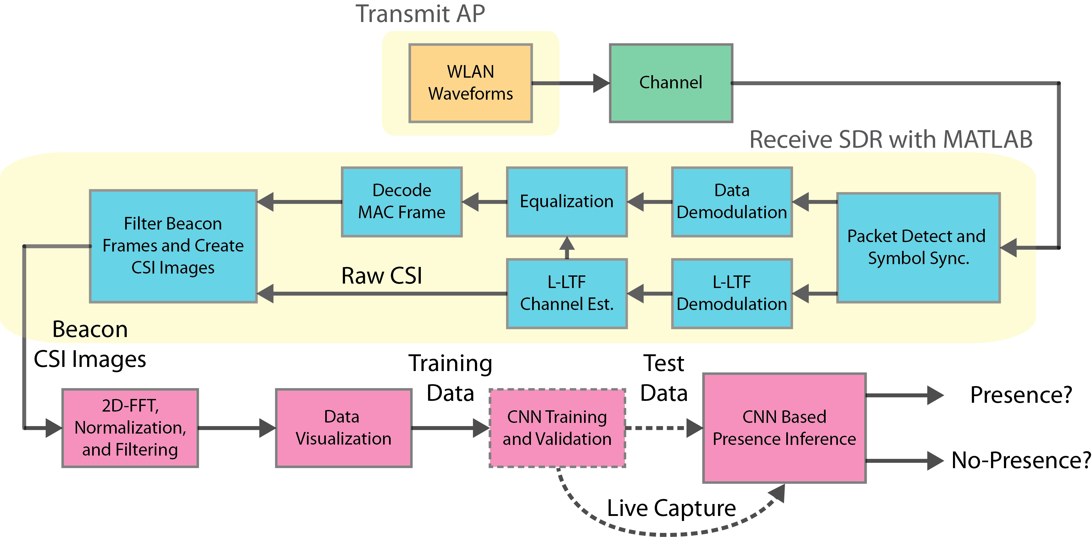
When you use an SDR, the system captures an over-the-air waveform and performs receiver processing in WLAN Toolbox to extract the CSI from beacon packets. It does the same for all the packets in a capture to form a numSubcarriers-by-rxsim.NumPacketsPerCapture raw CSI array. Repeat this process for multiple captures to create an array of images. When you create the training data, the system assigns "no-presence" or "presence" labels to the captures. It obtains the periodogram representation of the raw CSI image array by using 2D-FFT, applying [0 1] range scaling, and removing DC components along the and axes. CSI periodogram images make it easier to focus on the CSI changes caused by human motion by discarding the effects of imperfections in the hardware, software, or environment. This focus also improves the training performance. Next, you use the periodogram images as an input dataset for CNN training and validation. Finally, you use the trained CNN with live SDR captures to detect presence or test the performance of the CNN by using a subset of the prerecorded dataset. When capturing training data or performing live detection, you can visualize the magnitude spectrum and periodogram representation of the raw CSI.
This process was applied to obtain the prerecorded CSI dataset, which consists of 500 samples, with 250 labeled "no-presence" and 250 labeled "presence". When this dataset was being created, the rxsim.NumCaptures parameter was set to 250. An ADALM-Pluto SDR captured over-the-air beacon frames in a meeting room that contained furniture and had floor dimensions of 3m-by-3m. The beacon interval (rxsim.BeaconInterval) of the AP was set to 20 TUs. Two different human presence states were recorded: no presence (empty room) and presence (one person walking a random path).
Step 1: Create "no-presence" Data
In this section, you generate the "no-presence" data (dataNoPresence) and associated labels vector (labelNoPresence).
If you are using an SDR, make sure no human presence exists in the environment before you create the data. The
captureCSIDatasetfunction displays the current capture number, status, and timestamp (timestampNoPresence).If you are using the prerecorded dataset, the
loadCSIDatasetfunction generates thedataNoPresence,labelNoPresence,timestampNoPresenceparameters and visualizes the CSI dataset.
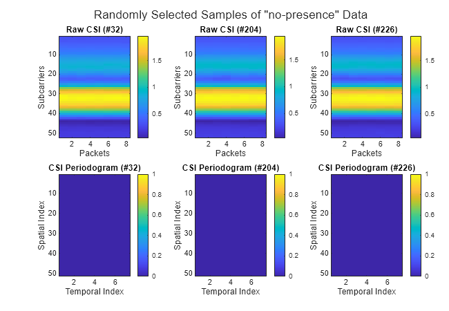
To generate the data, click Create "no-presence" Data. Two plots are generated for each capture:
Magnitude spectrum of the captured CSI. Although the captured CSI is a complex valued array, this example uses the magnitude response of the CSI for visualization.
CSI periodogram image.
In "no-presence" data, the power content of the CSI spreads over both axes of the periodogram representation due to the lack of time-domain disturbance induced by the motion.
if rxsim.UseSDR % Capture live CSI with SDR
    [dataNoPresence,labelNoPresence,timestampNoPresence] = captureCSIDataset(rxsim,"no-presence");
else % No SDR hardware, load CSI dataset
    [dataNoPresence,labelNoPresence,timestampNoPresence] = loadCSIDataset("dataset-no-presence.mat","no-presence");
end
Dimensions of the no-presence dataset (numSubcarriers x numPackets x numCaptures): [52 8 250]
Step 2: Create "presence" Data
In this section, you generate the "presence" data (dataPresence) and associated labels vector (labelPresence).
If you are capturing data with an SDR, make sure constant human motion exists in the environment before you create the data. Otherwise, the quality of the captured data could significantly worsen the performance during training and inference. The
captureCSIDatasetfunction displays the current capture number, status, timestamp (timestampPresence), and CSI visualization.If you are using the prerecorded dataset, the
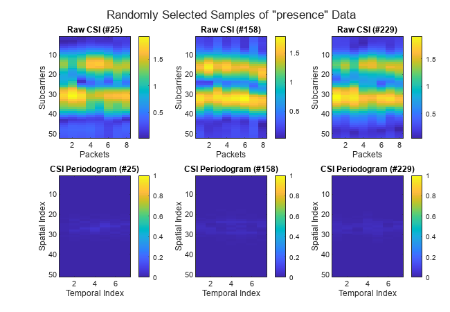
loadCSIDatasetfunction generates thedataPresence,labelPresence,timestampPresenceparameters and visualizes randomly selected samples of the data. The "presence" data in the prerecorded dataset was collected with a person walking constantly in the room for the duration of the capture.
The capture visualization techniques are the same as in step 1. For the "presence" data, the periodogram plot shows focus of the CSI power content in both axes near the low frequency region that corresponds to the center of the image.
if rxsim.UseSDR % Capture CSI with SDR
    [dataPresence,labelPresence,timestampPresence] = captureCSIDataset(rxsim,"presence");
else % No SDR hardware, load CSI dataset
    [dataPresence,labelPresence,timestampPresence] = loadCSIDataset("dataset-presence.mat","presence");
end
Dimensions of the presence dataset (numSubcarriers x numPackets x numCaptures): [52 8 250]
Step 3: Create and Train CNN
CNNs are one of the most computationally efficient, accurate, and scalable approaches to problems involving deep learning. Their predominant application is to deep learning tasks based on computer vision [3]. In this section, you define the CNN architecture and divide the data into training (dsTrain) and validation (dsValidation) datasets to evaluate the training and final network performance.
If you are using an SDR, you can evaluate the accuracy of the trained CNN using the live capture results. The example does not create a test set if you use an SDR.
If you are using the precaptured data, you can evaluate the performance of the trained CNN using a test set (
dsTest).
To create, train and validate the CNN click Create CNN and Train.
 trainRatio = 0.8;
numEpochs = 10;
sizeMiniBatch = 8;
trainRatio =  0.8;
numEpochs = 10;
sizeMiniBatch = 8;
Use the trainValTestSplit function to create array datastore objects dsTrain, dsValidation if you are using an SDR, and dsTest if you are using the precaptured data. This process is based on the trainRatio parameter. A training dataset (dsTrain), which comprises 80% of the whole dataset, updates the weights of the CNN to fit the general characteristics of the data. This process is based on the training labels contained in the array datastore object. A validation dataset (dsValidation), which comprises 10% of the whole dataset, ensures that the model is learning the general behavior of the system rather than memorizing the patterns in it. Finally, a test dataset (dsTest), which also comprises 10% of the whole dataset, evaluates the performance of the trained CNN using unseen samples of the data. If you are using an SDR, the size of dsValidation becomes 20% of the whole dataset, because the testing is based on the human presence status inferences of the trained CNN.
[dsTrain,dsValidation,dsTest,imageSize,classNames] = trainValTestSplit(rxsim.UseSDR,trainRatio,dataNoPresence,labelNoPresence,dataPresence,labelPresence);
CSI image size: [51   7]
Number of training images: 400
Number of validation images: 50
Number of test images: 50
The example uses CSI periodogram images with size (numSubcarriers-1)-by-(rxsim.NumPacketsPerCapture-1) as the training input. Use the Create Simple Deep Learning Neural Network for Classification (Deep Learning Toolbox) example to learn more about the individual layers and their roles in the architecture.
% Convolutional neural network (CNN) architecture
layers = [
    imageInputLayer(imageSize,'Normalization','none')

    convolution2dLayer(3,8,'Padding','same')
    batchNormalizationLayer
    reluLayer
    maxPooling2dLayer(2,'Stride',2)

    convolution2dLayer(3,16,'Padding','same')
    batchNormalizationLayer
    reluLayer
    maxPooling2dLayer(2,'Stride',2)

    convolution2dLayer(3,32,'Padding','same')
    batchNormalizationLayer
    reluLayer
    dropoutLayer(0.1)
    fullyConnectedLayer(numel(classNames))
    softmaxLayer]
layers =
  15x1 Layer array with layers:

     1   ''   Image Input           51x7x1 images
     2   ''   2-D Convolution       8 3x3 convolutions with stride [1  1] and padding 'same'
     3   ''   Batch Normalization   Batch normalization
     4   ''   ReLU                  ReLU
     5   ''   2-D Max Pooling       2x2 max pooling with stride [2  2] and padding [0  0  0  0]
     6   ''   2-D Convolution       16 3x3 convolutions with stride [1  1] and padding 'same'
     7   ''   Batch Normalization   Batch normalization
     8   ''   ReLU                  ReLU
     9   ''   2-D Max Pooling       2x2 max pooling with stride [2  2] and padding [0  0  0  0]
    10   ''   2-D Convolution       32 3x3 convolutions with stride [1  1] and padding 'same'
    11   ''   Batch Normalization   Batch normalization
    12   ''   ReLU                  ReLU
    13   ''   Dropout               10% dropout
    14   ''   Fully Connected       2 fully connected layer
    15   ''   Softmax               softmax
Specify the set of options for training the network. By default, this example trains the model on a GPU if one is available. Using a GPU requires the Parallel Computing Toolbox™ and a supported GPU device. For information on supported devices, see GPU Computing Requirements (Parallel Computing Toolbox) (Parallel Computing Toolbox).
% Training options
options = trainingOptions("adam", ...
    LearnRateSchedule="piecewise", ...
    InitialLearnRate=0.001, ... % learning rate
    MaxEpochs=numEpochs, ...
    MiniBatchSize=sizeMiniBatch, ...
    ValidationData=dsValidation, ...
    Shuffle="every-epoch", ...
    Metrics="accuracy",...
    ExecutionEnvironment="auto",...
    Verbose=true);
lossFcn = "crossentropy"; % cross-entropy loss for binary classification-based presence detection
Train the deep neural network net using the training dataset (dsTrain), network layers (layers), loss function (lossFcn), and the training options (options).
% Train the network
net = trainnet(dsTrain,layers,lossFcn,options);
Iteration Epoch TimeElapsed LearnRate TrainingLoss ValidationLoss TrainingAccuracy ValidationAccuracy
_________ _____ ___________ _________ ____________ ______________ ________________ __________________
0 0 00:00:03 0.001 0.69332 22
1 1 00:00:03 0.001 0.87107 50
50 1 00:00:06 0.001 0.010151 1.4619 100 50
100 2 00:00:10 0.001 0.012056 0.020318 100 100
150 3 00:00:12 0.001 0.0037492 0.0029605 100 100
200 4 00:00:13 0.001 0.0015092 0.00091004 100 100
250 5 00:00:16 0.001 1.5435 0.0048796 75 100
300 6 00:00:18 0.001 0.00093694 0.00067727 100 100
350 7 00:00:21 0.001 0.0030583 0.00052483 100 100
400 8 00:00:23 0.001 0.00011237 0.00025645 100 100
450 9 00:00:24 0.001 0.00055007 0.00027331 100 100
500 10 00:00:26 0.001 0.00010339 0.000141 100 100
Training stopped: Max epochs completed
Step 4: Evaluate Performance
In this section, you evaluate the performance of the neural network using training data or live inference with an SDR.
If you are using an SDR, this example uses the
livePresenceDetectionfunction to capture over-the-air beacons and infer human presence ("no-presence" or "presence") using the trained CNN that is for each capture. The function plots the instantaneous raw CSI and CSI periodogram plots, as described in steps 1 and 2, for each capture. The timestamped results for the 10 latest predictions are plotted. By default,livePresenceDetectionruns for 20 captures. You can setnumCapturesargument to any integer value. For continuous capturing, you can setnumCapturestoInf. The function returns results in the 1-by-2 cell arraysensingResults.The first element is the prediction results and the second element is the timestamps. Note thatsensingResultswill not be created iflivePresenceDetectionis in the continuous capturing mode.If you are using the prerecorded data, this example uses the
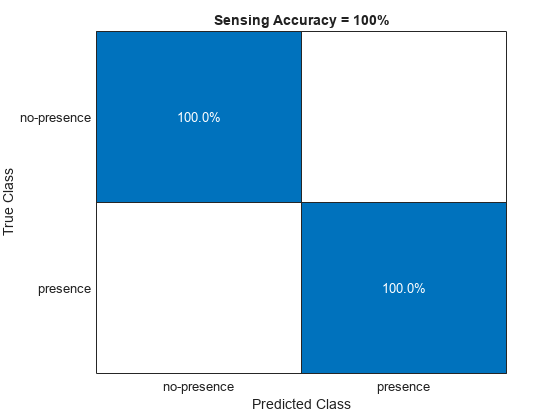
testPresenceDetectionfunction to generate a confusion matrix in which the rows correspond to the ground truth values ("no-presence" or "presence") and the columns correspond to the CNN predictions ("no-presence" or "presence"). The diagonal elements represent the percentage of samples that are correctly classified. The off-diagonal elements are the percentage of incorrectly classified observations. The sensing accuracy value is calculated using thedsTestand returned insensingResults.
To run the evaluation, click Evaluate Performance.
if rxsim.UseSDR % Predict movement from the live SDR captures
    sensingResults = livePresenceDetection(rxsim,net,classNames,20);
else % Predict movement by using the test set
    sensingResults = testPresenceDetection(dsTest,net,classNames);
end
Local Functions
These local functions assist with SDR setup.
function rxsim = setupSDR(rxsim)
    % Set up hardware
    if isfield(rxsim,'SDRObj')
        rx = rxsim.SDRObj;
    else
        rx = hSDRReceiver(rxsim.DeviceName);
    end
    if rxsim.UsePD && matches(rxsim.DeviceName,hSDRBase.ListOfWTConfigurations)
        % Set up preamble detector
        if ~isa(rx,'preambleDetector')
            % Delete existing WT radio config object if any
            delete(rx.SDRObj);
            rx = preambleDetector(rxsim.DeviceName);
        end
        wsd = hWLANOFDMDescriptor(Band=rxsim.FrequencyBand,Channel=rxsim.ChannelNumber,ChannelBandwidth="CBW20");
        rx = configureDetector(wsd,rx);
        rx.RadioGain = rxsim.RadioGain;
        rx.CaptureDataType = "single";

        % Tune Preamble Detector
        rx.ThresholdMethod = "adaptive";
        rx.AdaptiveThresholdGain = rxsim.ThresholdGain;
        rx.AdaptiveThresholdOffset = rxsim.ThresholdOffset;
    else
        % Set up SDR receiver object
        if isa(rx,'preambleDetector')
            delete(rx)
        end
        rx = hSDRReceiver(rxsim.DeviceName);
        rx.Gain = rxsim.RadioGain;
        rx.SampleRate = 20e6; % Configured for 20 MHz since this is beacon transmission bandwidth
        rx.CenterFrequency = wlanChannelFrequency(rxsim.ChannelNumber,rxsim.FrequencyBand);
        rx.OutputDataType = "single";
    end
    rxsim.SDRObj = rx;
end
References
[1] IEEE P802.11 - TASK GROUP BF (WLAN SENSING), https://www.ieee802.org/11/Reports/tgbf_update.htm.
[2] IEEE 802.11-21/0407r2 - Multi-Band WiFi Fusion for WLAN Sensing, March 2021, https://mentor.ieee.org/802.11/dcn/21/11-21-0407-00-00bf-multi-band-wifi-fusion-for-wlan-sensing.pptx.
[3] Y. Lecun, L. Bottou, Y. Bengio and P. Haffner, "Gradient-based learning applied to document recognition," in Proceedings of the IEEE, Vol. 86, No. 11, pp. 2278–2324, Nov. 1998, doi: 10.1109/5.726791.
Related Topics
You can also select a web site from the following list:
Americas
- América Latina (Español)
- Canada (English)
- United States (English)
Europe
- Belgium (English)
- Denmark (English)
- Deutschland (Deutsch)
- España (Español)
- Finland (English)
- France (Français)
- Ireland (English)
- Italia (Italiano)
- Luxembourg (English)
- Netherlands (English)
- Norway (English)
- Österreich (Deutsch)
- Portugal (English)
- Sweden (English)
- Switzerland
- United Kingdom (English)