Three-Dimensional Indoor Positioning with 802.11az Fingerprinting and Deep Learning

Introduction

The IEEE 802.11az Wi-Fi™ standard [1], commonly referred to as next generation positioning (NGP), provides physical layer features that enable enhanced ranging and positioning using classical techniques.

Classical techniques rely on line-of-sight (LOS) conditions to effectively extract temporal information, such as time of arrival (ToA), or spatial information, such as angle of arrival (AoA), from a multipath signal to compute a distance or range between devices. When the range between a minimum of three devices can be measured, trilateration can be used to compute a position estimate. For more information about how to use classical ranging and positioning techniques, see the 802.11az Positioning Using Super-Resolution Time of Arrival Estimation example.

Fingerprinting and deep learning techniques can be used in Wi-Fi positioning systems to achieve sub-meter accuracies even in non-line-of-sight (NLOS) multipath environments [2]. A fingerprint typically contains channel state information (CSI), such as a received signal strength indicator (RSSI) or a channel estimate from a received signal, measured at a specific location in an environment [3].

During the training phase of the network, the example creates a database by sampling the channel fingerprints at multiple known locations in an environment. The network estimates the user location based on a signal received at an unknown location by using the database as a reference.

This example creates a data set of CIR fingerprints by using 802.11az signals in an indoor environment, labeling each fingerprint with its location information for a channel bandwidth of 40 MHz. The example trains a CNN to predict STA locations by using a subset of the fingerprints, then evaluates the performance of the trained model by generating predictions of STA locations based on their CIR fingerprint remainder of the data set.

For simplicity, this example uses a small data set, which results in a short simulation time. For more accurate results, use a larger data set. The example provides pretrained models to show the high levels of performance that can be achieved with more training data.

Simulation Parameters

Indoor Propagation Environment

Generate training data for an indoor office environment specified by the office.stl file.

mapFileName = "office.stl";
viewer = siteviewer("SceneModel",mapFileName,"Transparency",0.25);

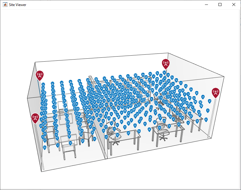
The example places four access points (APs) and a number of STAs that you specify in this environment. The example generates the fingerprints based on the propagation channel defined by the environment, then generates the associated channel impulse response by using ray tracing techniques. For more information on ray tracing for indoor environments, see the Indoor MIMO-OFDM Communication Link Using Ray Tracing example.

AP and STA Parameters

Select the size of the transmit and receive antenna arrays, and the channel bandwidth. These parameters control the quantity of data and its resolution within each fingerprint. Larger antenna arrays produce more channel realizations and more CIRs per fingerprint. A higher bandwidth increases the sample rate of the CIR, capturing it in more detail. Changing these parameters makes the data set incompatible with the pretrained models, as the dimensions of each fingerprint must match the shape of the model input layer.

S = RandStream("mt19937ar","Seed",5489); % Set the RNG for reproducibility
RandStream.setGlobalStream(S);

txArraySize = [4 1]; % Linear transmit array
rxArraySize = [4 1]; % Linear receive array
chanBW      = "CBW40";

Specify the number of STAs used to map the environment and the distribution of STAs. To distribute STAs uniformly in each dimension as an evenly spaced grid, set distribution to uniform. To distribute STAs randomly within the environment, set distribution to random.

When you distribute the STAs uniformly, the example determines the number of STAs by using the value of staSeparation, which measures the distance, in meters, between STAs in all dimensions.

When you randomly distribute STAs, specify the number of STAs by setting the value of numSTAs.

distribution  = "uniform";
staSeparation = 0.5; % STA separation in meters. This parameter is used only when the distribution is uniform.
numSTAs       = 500; % Number of STAs. This parameter is used only when the distribution is random.

Localization and Positioning

The parameter task determines whether the example performs fingerprinting-based localization or 3D positioning [4]. Fingerprinting-based localization is a multi-class classification task, which predicts the discrete area of the map at which an STA is located. Fingerprinting-based localization is useful for tasks where the detection of the discrete position of an STA, for example, the room of a building or an aisle in a store, is sufficient. 3D positioning is a regression task in which the output of the model is the predicted position of an STA. Positioning can estimate the exact location of the user but can have a higher error for positions across an area when compared to localization.

task = "localization";

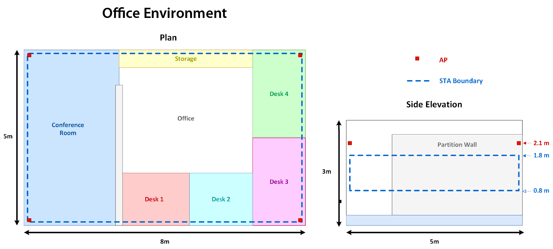
Fingerprinting-based localization task determines the general location of an STA, rather than its precise 3D location. The following diagram shows the layout of the small office with discrete areas used as classes for localization. The red square markers indicate the locations of the APs. The blue dashed box represents the area where the example distributes the STAs during the training process. The example restricts the height of the STAs to a range between 0.8 and 1.8 meters. This range represents a realistic set of values for portable consumer devices. This constraint also minimizes the chance of STAs being placed in unreachable positions.

Training Data Synthesis

This section shows how to synthesize the data set for training the CNN.

Generate AP and STA Positions

Generate the AP and STA objects and visualize them in the indoor scenario. If you use a file other than office.stl, you must adjust the AP and STA locations within the dlPositioningCreateEnvironment function to fit the new environment.

if distribution == "uniform"
    [APs,STAs] = dlPositioningCreateEnvironment(txArraySize,rxArraySize,staSeparation,"uniform");
else
    [APs,STAs] = dlPositioningCreateEnvironment(txArraySize,rxArraySize,numSTAs,"random");
end
show(APs)
show(STAs,"ShowAntennaHeight",false,"IconSize",[16 16]);
disp(['Simulating a scenario with ',num2str(width(APs)),' APs and ',num2str(width(STAs)),' STAs with ',char(distribution),' distribution...'])

Simulating a scenario with 4 APs and 480 STAs with uniform distribution...

Generate Channel Characteristics by Using Ray Tracing Techniques

Set the parameters of the ray propagation model. This example considers only LOS and first-order reflections by setting the MaxNumReflections parameter to 1.Increasing the maximum number of reflections increases the simulation time. To consider only LOS propagation, set the MaxNumReflections property to 0.

pm = propagationModel("raytracing", ...
    "CoordinateSystem","cartesian", ...
    "SurfaceMaterial","wood", ...
    "MaxNumReflections",1);

Perform ray tracing analysis for all AP-STA pairs. The raytrace function returns the generated rays in a cell array of size $$N_{\text{AP}}$$-by-$$N_{\text{STA}}$$, where $$N_{\text{AP}}$$ is the number of APs and $$N_{\text{STA}}$$ is the number of STAs.

% Perform ray tracing for all transmitters and receivers in parallel
rays = raytrace(APs,STAs,pm,"Map",mapFileName);
size(rays)

ans = 1×2

     4   480

Visualize the calculated rays between all APs and a single STA. The color represents the associated path loss in dB.

hide(STAs);
show(STAs(ceil(width(STAs)/2)),'IconSize',[32 32]);
plot([rays{:,ceil(width(rays)/2)}],'ColorLimits',[50 95]);

Generate 802.11az CIR Fingerprint Features and Labels

This section shows how to compute the CIRs for each AP-STA pair by using the calculated rays. This diagram shows the processing chain that the example uses to generate the CIRs.

Each AP transmits an 802.11az packet through a noisy channel, and each STA receives the packet. The example assumes that each STA can differentiate between APs, and that no interference occurs between APs.

Packet reception at a location fails if the path between the location and an AP, or if synchronization fails due to low SNR. In this case, the generated CIR is a vector of zeros.

This example uses the magnitude of each multipath component in the CIR as training data. Therefore, the generated CIRs are real-valued. The example stores the CIRs in a four-dimensional array of size $$N_{\text{s}}$$-by-$$N_{\text{tx}\text{-}\text{rx}}$$-by-$$N_{\text{AP}}$$-by-$$N_{\text{r}}$$.

The example trains the CNN by combining these features with labels of the STA position or location names.

To simulate variations in the environment, repeat the fingerprinting process under different noise conditions by specifying a range of SNR values.

snrs = [10 15 20];

Configure the waveform parameters. In particular, set the number of space-time streams (STSs) to the size of the transmit antenna array to ensure that the signal from each transmit antenna contributes to the fingerprint of an STA during channel estimation.

cfg = heRangingConfig('ChannelBandwidth',chanBW, ...
    "NumTransmitAntennas",prod(txArraySize), ...
    "SecureHELTF",false);
cfg.User{1}.NumSpaceTimeStreams = prod(txArraySize);

Generate the data set.

[features,labels] = dlPositioningGenerateDataSet(rays,STAs,APs,cfg,snrs);

Generating Dataset: 10% complete.
Generating Dataset: 20% complete.
Generating Dataset: 30% complete.
Generating Dataset: 40% complete.
Generating Dataset: 50% complete.
Generating Dataset: 60% complete.
Generating Dataset: 70% complete.
Generating Dataset: 80% complete.
Generating Dataset: 90% complete.
Generating Dataset: 100% complete.

Deep Learning

Deep learning uses neural networks to approximate functions across a diverse range of domains. A CNN is a neural network architecture that uses two-dimensional multichannel images. CNNs preserve and learn features from spatial aspects of the data. The deep learning workflow comprises these steps.

Define Training Data

Neural networks are powerful models that can fit a variety of data. To validate results, split the data set into 80% training data and 20% validation data. Training data is the data that the model learns to fit by adjusting its weighted parameters based on the error of its predictions. Validation data is the data that the example uses to ensure that the model is performing as expected on unseen data and not overfitting the training data.

[training,validation] = dlPositioningSplitDataSet(features,labels,0.2);

Define Neural Network Model

A typical CNN consists of seven main layers.

You can form a deep network by arranging layers from these classes and repeating them in blocks. The CNN in this example consists of four blocks, each with a convolution, batch normalization, ReLU, and average pooling layer. The example adds dropout regularization (20%) before the final layers. This architecture is similar to that of the CNN used in the Train Convolutional Neural Network for Regression (Deep Learning Toolbox) example, which predicts the rotated positions of handwritten digit images and demonstrates the diverse applications of deep learning models with minimal changes to their parameters.

Construct the CNN.

layers = [
    
    imageInputLayer(size(training.X, 1:3))

    convolution2dLayer(3,256,"Padding","same")
    batchNormalizationLayer
    reluLayer
    
    averagePooling2dLayer(2,"Stride",2,"Padding","same")
    
    convolution2dLayer(3,256,"Padding","same")
    batchNormalizationLayer
    reluLayer
    
    averagePooling2dLayer(2,"Stride",2,"Padding","same")

    convolution2dLayer(3,256,"Padding","same")
    batchNormalizationLayer
    reluLayer
    
    averagePooling2dLayer(2,"Stride",2,"Padding","same")
  
    convolution2dLayer(3,256,"Padding","same")
    batchNormalizationLayer
    reluLayer
    
    averagePooling2dLayer(2,"Stride",2,"Padding","same")
   
    dropoutLayer(0.2)];

Specify the size of the output layer and the activation function for the output, depending on the selected task.

if task == "localization" % classification
    layers = [
        layers
        fullyConnectedLayer(7)
        softmaxLayer];
    lossFcn = "crossentropy";
    trainingMetric = "accuracy";
else % positioning (regression)
    layers = [
        layers
        fullyConnectedLayer(3)];
    lossFcn = "mse";
    trainingMetric = "rmse";
end

Match the labels given to the network with the expected model output for each task. The features are an image of CIR fingerprints for both tasks.

if task == "localization" % classification
    valY = validation.Y.classification;
    trainY = training.Y.classification;
else % positioning (regression)
    valY = validation.Y.regression;
    trainY = training.Y.regression;
end

Configure Learning Process and Train Model

Set the number of training data samples that the model evaluates during each training iteration. Increase the number of samples when using a larger data set.

miniBatchSize = 32;

Set the validation frequency so that the network is validated about once per epoch. The network evaluates the unseen samples to test generalization at the end of each validation period.

validationFrequency = floor(size(training.X,4)/miniBatchSize);

Specify the options that control the training process. The number of epochs controls how many times the example trains the model consecutively on the full training data set. By default, the example trains the model on a GPU if one is available. Using a GPU required Parallel Computing Toolbox™ and a supported GPU device. For information on supported devices, see GPU Computing Requirements (Parallel Computing Toolbox).

options = trainingOptions("adam", ...
    "MiniBatchSize",miniBatchSize, ...
    "MaxEpochs",3, ...
    "InitialLearnRate",1e-4,...
    "Metrics",trainingMetric,...
    "Shuffle","every-epoch", ...
    "ValidationData",{validation.X,valY'}, ...
    "ValidationFrequency",validationFrequency, ...
    "Verbose",true, ...
    "ResetInputNormalization",true, ...
    "ExecutionEnvironment","auto");

Train the model.

net = trainnet(training.X,trainY.',layers,lossFcn,options);

    Iteration    Epoch    TimeElapsed    LearnRate    TrainingLoss    ValidationLoss    TrainingAccuracy    ValidationAccuracy
    _________    _____    ___________    _________    ____________    ______________    ________________    __________________
            0        0       00:00:06       0.0001                            1.9462                                      6.25
            1        1       00:00:07       0.0001          2.3813                                 3.125                      
           36        1       00:00:37       0.0001          1.1718            2.0518              59.375                6.5972
           50        2       00:00:49       0.0001         0.87043                                78.125                      
           72        2       00:01:08       0.0001         0.90884            1.3967              71.875                51.389
          100        3       00:01:31       0.0001          1.0756                                71.875                      
          108        3       00:01:39       0.0001          1.1772           0.84391                  50                71.181
Training stopped: Max epochs completed

Evaluate Model Performance

Investigate the model performance by examining predicted values for the validation data. Predict labels by passing the validation set features through the network, then evaluate the performance of the network by comparing the predicted labels with the validation set labels.

if task == "localization"
    YScores = minibatchpredict(net,validation.X);
    YPred = scores2label(YScores,categories(labels.class));
else % positioning
    YPred = minibatchpredict(net,validation.X);
end

Generate a visual and statistical view of the results.

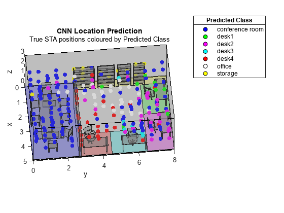
For localization, the dlPositioningPlotResults function generates a three-dimensional map, which displays the true locations of STAs. The color assigned to each STA denotes its predicted location. The function also generates a confusion matrix in which the rows correspond to the predicted class and the columns correspond to the true class. The diagonal cells correspond to observations that are correctly classified. The off-diagonal cells correspond to incorrectly classified observations. If the network performs well, elements in the main diagonal are significantly larger than the other matrix elements.

For positioning, the color assigned to each STA denotes the distance error of the predicted position. The function also generates a cumulative distribution function (CDF). The y-axis measures the proportion of the data for which the measured distance error is less than or equal to the corresponding value on the x-axis.

This example uses a small data set and limited training period, which produces modest results. You can obtain more accurate results by using a CNN pretrained with a large data set.

metric = dlPositioningPlotResults(mapFileName,validation.Y,YPred,task);

Pretrained Model

Download a CNN for positioning and localization pretrained with a large data set from https://www.mathworks.com/supportfiles/spc/wlan/Positioning80211azExample/pretrained_networks_R2024b.zip. This zip file contains two MAT files:

All models were trained for 100 epochs with a miniBatchSize value of 256 on a data set of fingerprints from a uniform distribution of STAs with a staSeparation value of 0.1. The bandwidth was 40 MHz with four-antenna linear arrays in the transmitter and receiver (4$$\times$$4 MIMO).

To explore the performance of these pretrained models, download and extract the zip file, load the appropriate MAT file into the workspace, and run the Evaluate Model Performance section again.

Effect of Antenna Array Size

The pretrained models show that an increased number of STAs and training epochs improve performance. This section shows the effect of antenna arrays on performance for a channel bandwidth of 40 MHz. These results were generated by training a model for 100 epochs with a miniBatchSize value of 256 with a data set compiled from a uniform distribution of STAs sampled at intervals of 0.1 meters, in which each STA and AP contained a four-element linear antenna array.

These figures show the impact of the number of transmit and receive antennas. The accuracy increases for larger antenna arrays due to the presence of more channel information. For example, a 4$$\times$$4 channel contains 16 channel realizations, whereas a 2$$\times$$2 channel contains only four. As expected, the CNN performs better when trained with more data.

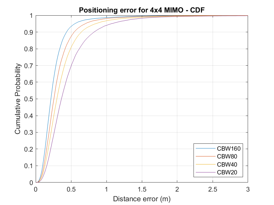
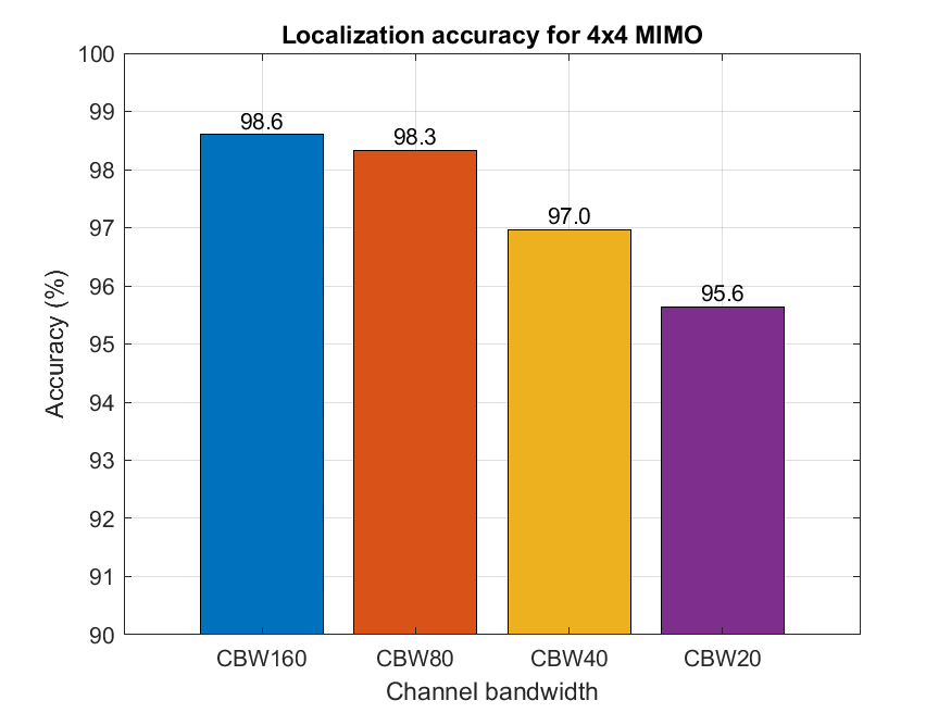
These results were generated with data samples which were not used to train the CNNs. If data samples used to train the CNN are also used to evaluate performance the results may differ.

References

IEEE Std 802.11az™-2022. IEEE Standard for Information technology— Telecommunications and information exchange between systems Local and metropolitan area networks— Specific requirements - Amendment 3: Enhancements for positioning.
Kokkinis, Akis, Loizos Kanaris, Antonio Liotta, and Stavros Stavrou, “RSS Indoor Localization Based on a Single Access Point”, Sensors 19, no. 17 (August 27, 2019): 3711. https://doi.org/10.3390/s19173711.
Wang, Xuyu, Lingjun Gao, Shiwen Mao, and Santosh Pandey, “CSI-Based Fingerprinting for Indoor Localization: A Deep Learning Approach”, IEEE Transactions on Vehicular Technology, 2016, 763–776. https://doi.org/10.1109/TVT.2016.2545523.
Groves, Paul D. "Principles of GNSS, Inertial, and Multisensor Integrated Navigation Systems", Boston: Artech House, 2008.