CSI Feedback with Autoencoders

This example uses:

This example shows how to use an autoencoder neural network to compress downlink channel state information (CSI) over a clustered delay line (CDL) channel. CSI feedback is in the form of a raw channel estimate array.

Introduction

In conventional 5G radio networks, CSI parameters are quantities related to the state of a channel that are extracted from the channel estimate array. The CSI feedback includes several parameters, such as the Channel Quality Indication (CQI), the precoding matrix indices (PMI) with different codebook sets, and the rank indicator (RI). The UE uses the CSI reference signal (CSI-RS) to measure and compute the CSI parameters. The user equipment (UE) reports CSI parameters to the access network node (gNB) as feedback. Upon receiving the CSI parameters, the gNB schedules downlink data transmissions with attributes such as modulation scheme, code rate, number of transmission layers, and MIMO precoding. This figure shows an overview of a CSI-RS transmission, CSI feedback, and the transmission of downlink data that is scheduled based on the CSI parameters.

The UE processes the channel estimate to reduce the amount of CSI feedback data. As an alternative approach, the UE compresses and feeds back the channel estimate array. After receipt, the gNB decompresses and processes the channel estimate to determine downlink data link parameters. The compression and decompression can be achieved using an autoencoder neural network [1, 2]. This approach eliminates the use of existing quantized codebook and can improve overall system performance.

This example uses a 5G downlink channel with these system parameters.

txAntennaSize = [2 2 2 1 1]; % rows, columns, polarizations, panels
rxAntennaSize = [2 1 1 1 1]; % rows, columns, polarizations, panels
rmsDelaySpread = 300e-9;     % s
maxDoppler = 5;              % Hz
nSizeGrid = 52;              % Number resource blocks (RB)
                             % 12 subcarriers per RB
subcarrierSpacing = 15;      % 15, 30, 60, 120 kHz
numTrainingChEst = 15000;

% Carrier definition
carrier = nrCarrierConfig;
carrier.NSizeGrid = nSizeGrid;
carrier.SubcarrierSpacing = subcarrierSpacing

carrier = 
  nrCarrierConfig with properties:

                NCellID: 1
      SubcarrierSpacing: 15
           CyclicPrefix: 'normal'
              NSizeGrid: 52
             NStartGrid: 0
                  NSlot: 0
                 NFrame: 0
    IntraCellGuardBands: [0×2 double]

   Read-only properties:
         SymbolsPerSlot: 14
       SlotsPerSubframe: 1
          SlotsPerFrame: 10

autoEncOpt.NumSubcarriers = carrier.NSizeGrid*12;
autoEncOpt.NumSymbols = carrier.SymbolsPerSlot;
autoEncOpt.NumTxAntennas = prod(txAntennaSize);
autoEncOpt.NumRxAntennas = prod(rxAntennaSize);

Generate and Preprocess Data

The first step of designing an AI-based system is to prepare training and testing data. For this example, generate simulated channel estimates and preprocess the data. Use 5G Toolbox™ functions to configure a CDL-C channel.

waveInfo = nrOFDMInfo(carrier);
samplesPerSlot = ...
  sum(waveInfo.SymbolLengths(1:waveInfo.SymbolsPerSlot));

channel = nrCDLChannel;
channel.DelayProfile = 'CDL-C';
channel.DelaySpread = rmsDelaySpread;       % s
channel.MaximumDopplerShift = maxDoppler;   % Hz
channel.RandomStream = "Global stream";
channel.TransmitAntennaArray.Size = txAntennaSize;
channel.ReceiveAntennaArray.Size = rxAntennaSize;
channel.ChannelFiltering = false;           % No filtering for 
                                            % perfect estimate
channel.NumTimeSamples = samplesPerSlot;    % 1 slot worth of samples
channel.SampleRate = waveInfo.SampleRate;

Simulate Channel

Run the channel and get the perfect channel estimate, Hest.

[pathGains,sampleTimes] = channel();
pathFilters = getPathFilters(channel);
offset = nrPerfectTimingEstimate(pathGains,pathFilters);
Hest = nrPerfectChannelEstimate(carrier,pathGains,pathFilters, ...
  offset,sampleTimes);

The channel estimate matrix is an $[N_{subcarriers} N_{symbols} N_{rx} N_{tx}]$ array for each slot.

[nSub,nSym,nRx,nTx] = size(Hest)

nSub = 624

nSym = 14

nRx = 2

nTx = 8

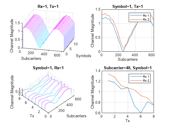
Plot the channel response. The upper left plot shows the channel frequency response as a function of time (symbols) for receive antenna 1 and transmit antenna 1. The lower left plot shows the channel frequency response as a function of transmit antennas for symbol 1 and receive antenna 1. The upper right plot shows the channel frequency response for all receive antennas for symbol 1 and transmit antenna 1. The lower right plot shows the change in channel magnitude response as a function of transmit antennas for all receive antennas for a subcarrier and symbol 1.

plotChannelResponse(Hest)

Preprocess Channel Estimate

Preprocess the channel estimate to reduce the size and convert it to a real-valued array. This figure shows the channel estimate reduction preprocess.

Channel estimate preprocessing

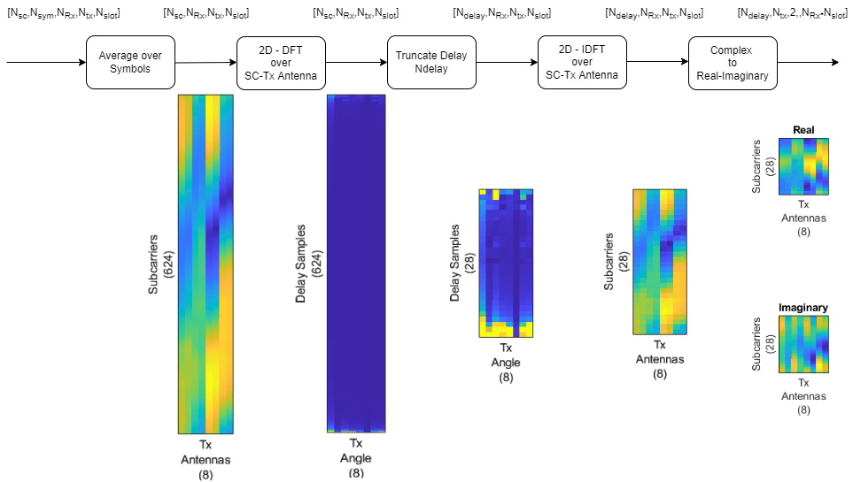
Assume that the channel coherence time is much larger than the slot time. Average the channel estimate over a slot and obtain a $[N_{subcarriers} 1 N_{rx} N_{tx}]$ array.

Hmean = mean(Hest,2);

To enable operation on subcarriers and Tx antennas, move the Tx and Rx antenna dimensions to the second and third dimensions, respectively.

Hmean = permute(Hmean,[1 4 3 2]);

To obtain the delay-angle representation of the channel, apply a 2-D discrete Fourier transform (DFT) over subcarriers and Tx antennas for each Rx antenna and slot. To demonstrate the workflow and reduce runtime, this subsection processes Rx channel 1 only.

Hdft2 = fft2(Hmean(:,:,1));

Since the multipath delay in the channel is limited, truncate the delay dimension to remove values that do not carry information. The sampling period on the delay dimension is $T_{d e l a y} = 1 / (N_{s u b c a r r i e r s} * F_{s s})$ , where $F_{s s}$ is subcarrier spacing. The expected RMS delay spread in delay samples is $τ_{R M S} / T_{d e l a y}$ , where $τ_{R M S}$ is the RMS delay spread of the channel in seconds.

Tdelay = 1/(autoEncOpt.NumSubcarriers*carrier.SubcarrierSpacing*1e3);
rmsTauSamples = channel.DelaySpread / Tdelay;
maxTruncationFactor = floor(autoEncOpt.NumSubcarriers / rmsTauSamples);

Truncate the channel estimate to an even number of samples that is 10 times the expected RMS delay spread. Increasing the truncationFactor value can decrease the performance loss due to preprocessing. But, doing so increases the neural network complexity, number of required training data points, and training time. A neural network with more learnable parameters might not converge to a better solution.

truncationFactor = 10;
maxDelay = round((channel.DelaySpread/Tdelay)*truncationFactor/2)*2

maxDelay = 28

autoEncOpt.MaxDelay = maxDelay;

Calculate the truncation indices and truncate the channel estimate.

midPoint = floor(nSub/2);
lowerEdge = midPoint - (nSub-maxDelay)/2 + 1;
upperEdge = midPoint + (nSub-maxDelay)/2;
Htemp = Hdft2([1:lowerEdge-1 upperEdge+1:end],:);

To get back to the subcarriers-Tx antennas domain, apply a 2-D inverse discrete Fourier transform (IDFT) to the truncated array [2]. This process effectively decimates the channel estimate in the subcarrier axis.

Htrunc = ifft2(Htemp);

Separate the real and imaginary parts of the channel estimate to obtain a $[N_{delay} N_{tx} 2]$ array.

HtruncReal = zeros(maxDelay,nTx,2);
HtruncReal(:,:,1) = real(Htrunc);
HtruncReal(:,:,2) = imag(Htrunc); %#ok<NASGU>

Plot the channel estimate signal through the preprocessing steps. Images are scaled to help visualization.

plotPreprocessingSteps(Hmean(:,:,1),Hdft2,Htemp,Htrunc,nSub,nTx, ...
  maxDelay)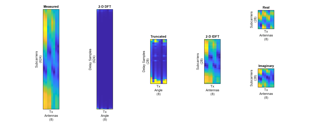

Prepare Data in Bulk

The helperCSINetTrainingData helper function generates numTrainingChEst of preprocessed $[N_{delay} N_{tx} 2]$ channel estimates by using the process described in this section. The function saves each $[N_{delay} N_{tx} 2]$ channel estimate as an individual file in the dataDir with the prefix of trainingDataFilePrefix. If Parallel Computing Toolbox™ is available, helperCSINetTrainingData function uses parfor to parallelize data generation. Data generation takes less than three minutes on a PC with Intel® Xeon® W-2133 CPU @ 3.60GHz and running in parallel on six workers.

dataDir = fullfile(exRoot(),"Data");
trainingDataFilePrefix = "nr_channel_est";
if validateTrainingFiles(dataDir,trainingDataFilePrefix, ...
    numTrainingChEst,autoEncOpt,channel,carrier) == false
  disp("Starting training data generation")
  tic
  autoEncOpt.Normalization = false;  % Do not normalize data yet
  
  helperCSINetTrainingData(dataDir,trainingDataFilePrefix, ...
    numTrainingChEst,carrier,channel,autoEncOpt);
  t = seconds(toc);
  t.Format = "hh:mm:ss";
  disp(string(t) + " - Finished training data generation")
end

Starting training data generation

Starting parallel pool (parpool) using the 'Processes' profile ...
19-Mar-2024 09:00:24: Job Queued. Waiting for parallel pool job with ID 4 to start ...
Connected to parallel pool with 6 workers.
6 workers running
00:00:16 -  8% Completed
00:00:31 - 16% Completed
00:00:47 - 24% Completed
00:01:03 - 32% Completed
00:01:18 - 40% Completed
00:01:31 - 48% Completed
00:01:45 - 56% Completed
00:02:00 - 64% Completed
00:02:17 - 72% Completed
00:02:33 - 80% Completed
00:02:53 - 88% Completed
00:03:07 - 96% Completed
Parallel pool using the 'Processes' profile is shutting down.

00:05:33 - Finished training data generation

Create a signalDatastore object to access the data. The signal datastore uses individual files for each data point.

sds = signalDatastore( ...
  fullfile(dataDir,"processed",trainingDataFilePrefix+"_*"));

Load data into memory, calculate the mean value and standard deviation, and then use the mean and standard deviation values to normalize the data.

HtruncRealCell = readall(sds);
HtruncReal = cat(4,HtruncRealCell{:});
meanVal = mean(HtruncReal,'all')

meanVal = single
    -0.0563

stdVal = std(HtruncReal,[],'all')

stdVal = single
    16.0602

Separate the data into training, validation, and test sets. Also, normalize the data to achieve zero mean and a target standard deviation of 0.0212, which restricts most of the data to the range of [-0.5 0.5].

N = size(HtruncReal, 4);
numTrain = floor(N*10/15)

numTrain = 10000

numVal = floor(N*3/15)

numVal = 3000

numTest = floor(N*2/15)

numTest = 2000

targetStd = 0.0212;
HTReal = (HtruncReal(:,:,:,1:numTrain)-meanVal) ...
  /stdVal*targetStd+0.5;
HVReal = (HtruncReal(:,:,:,numTrain+(1:numVal))-meanVal) ...
  /stdVal*targetStd+0.5;
HTestReal = (HtruncReal(:,:,:,numTrain+numVal+(1:numTest))-meanVal) ...
  /stdVal*targetStd+0.5;
autoEncOpt.MeanVal = meanVal;
autoEncOpt.StdValue = stdVal;
autoEncOpt.TargetSTDValue = targetStd;

Define and Train Neural Network Model

The second step of designing an AI-based system is to define and train the neural network model.

Define Neural Network

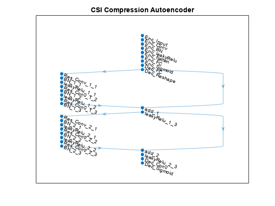
This example uses a modified version of the autoencoder neural network proposed in [1].

inputSize = [maxDelay nTx 2];  % Third dimension is real and imaginary parts
nLinear = prod(inputSize);
nEncoded = 64;

autoencoderNet = dlnetwork([ ...
    % Encoder
    imageInputLayer(inputSize,"Name","Htrunc", ...
      "Normalization","none","Name","Enc_Input")

    convolution2dLayer([3 3],2,"Padding","same","Name","Enc_Conv")
    batchNormalizationLayer("Epsilon",0.001,"Name","Enc_BN")
    leakyReluLayer(0.3,"Name","Enc_leakyRelu")

    flattenLayer("Name","Enc_flatten")

    fullyConnectedLayer(nEncoded,"Name","Enc_FC")

    sigmoidLayer("Name","Enc_Sigmoid")

    % Decoder
    fullyConnectedLayer(nLinear,"Name","Dec_FC")

    functionLayer(@(x)dlarray(reshape(x,maxDelay,nTx,2,[]),'SSCB'), ...
      "Formattable",true,"Acceleratable",true,"Name","Dec_Reshape")
    ]);

autoencoderNet = ...
  helperCSINetAddResidualLayers(autoencoderNet, "Dec_Reshape");

autoencoderNet = addLayers(autoencoderNet, ...
    [convolution2dLayer([3 3],2,"Padding","same","Name","Dec_Conv") ...
    sigmoidLayer("Name","Dec_Sigmoid")]);
autoencoderNet = ...
  connectLayers(autoencoderNet,"leakyRelu_2_3","Dec_Conv");

figure
plot(autoencoderNet)
title('CSI Compression Autoencoder')

Train Neural Network

Set the training options for the autoencoder neural network and train the network using the trainnet (Deep Learning Toolbox) function. Training takes less than 13 minutes on an Intel® Xeon® W-2133 CPU @ 3.60GHz with NVIDIA GeForce RTX 3080 GPU. Set trainNow to false to load the pretrained network. Note that the saved network works for the following settings. If you change any of these settings, set trainNow to true.

txAntennaSize = [2 2 2 1 1]; % rows, columns, polarizations, panels
rxAntennaSize = [2 1 1 1 1]; % rows, columns, polarizations, panels
rmsDelaySpread = 300e-9;     % s
maxDoppler = 5;              % Hz
nSizeGrid = 52;              % Number resource blocks (RB)
                             % 12 subcarriers per RB
subcarrierSpacing = 15;

trainNow = false;

miniBatchSize = 1000;
options = trainingOptions("adam", ...
    InitialLearnRate=0.01, ...
    LearnRateSchedule="piecewise", ...
    LearnRateDropPeriod=156, ...
    LearnRateDropFactor=0.5916, ...
    Epsilon=1e-7, ...
    MaxEpochs=1000, ...
    MiniBatchSize=miniBatchSize, ...
    Shuffle="every-epoch", ...
    ValidationData={HVReal,HVReal}, ...
    ValidationFrequency=20, ...
    Metrics="rmse", ...
    Verbose=true, ...
    ValidationPatience=20, ...
    OutputNetwork="best-validation-loss", ...
    ExecutionEnvironment="auto", ...
    Plots='none') %#ok<NASGU>

options = 
  TrainingOptionsADAM with properties:

             GradientDecayFactor: 0.9000
      SquaredGradientDecayFactor: 0.9990
                         Epsilon: 1.0000e-07
                InitialLearnRate: 0.0100
                       MaxEpochs: 1000
               LearnRateSchedule: 'piecewise'
             LearnRateDropFactor: 0.5916
             LearnRateDropPeriod: 156
                   MiniBatchSize: 1000
                         Shuffle: 'every-epoch'
                      WorkerLoad: []
             CheckpointFrequency: 1
         CheckpointFrequencyUnit: 'epoch'
                  SequenceLength: 'longest'
        PreprocessingEnvironment: 'serial'
                L2Regularization: 1.0000e-04
         GradientThresholdMethod: 'l2norm'
               GradientThreshold: Inf
                         Verbose: 1
                VerboseFrequency: 50
                  ValidationData: {[28×8×2×3000 single]  [28×8×2×3000 single]}
             ValidationFrequency: 20
              ValidationPatience: 20
             ObjectiveMetricName: 'loss'
                  CheckpointPath: ''
            ExecutionEnvironment: 'auto'
                       OutputFcn: []
                         Metrics: 'rmse'
                           Plots: 'none'
            SequencePaddingValue: 0
        SequencePaddingDirection: 'right'
                InputDataFormats: "auto"
               TargetDataFormats: "auto"
         ResetInputNormalization: 1
    BatchNormalizationStatistics: 'auto'
                   OutputNetwork: 'best-validation-loss'
                    Acceleration: "auto"

lossFunc = @(x,t) nmseLossdB(x,t);

Use the normalized mean squared error (NMSE) between the network inputs and outputs in dB as the training loss function to find the best set of weights for the autoencoder.

if trainNow
  [net,trainInfo] = ...
    trainnet(HTReal,HTReal,autoencoderNet,lossFunc,options); %#ok<UNRCH> 
  save("csiTrainedNetwork_" ...
    + string(datetime("now","Format","dd_MM_HH_mm")), ...
    'net','trainInfo','options','autoEncOpt')
else
  helperCSINetDownloadData()
  autoEncOptCached = autoEncOpt;
  load("csiTrainedNetwork",'net','trainInfo','options','autoEncOpt')
  if autoEncOpt.NumSubcarriers ~= autoEncOptCached.NumSubcarriers ...
      || autoEncOpt.NumSymbols ~= autoEncOptCached.NumSymbols ...
      || autoEncOpt.NumTxAntennas ~= autoEncOptCached.NumTxAntennas ...
      || autoEncOpt.NumRxAntennas ~= autoEncOptCached.NumRxAntennas ...
      || autoEncOpt.MaxDelay ~= autoEncOptCached.MaxDelay
    error("CSIExample:Missmatch", ...
      "Saved network does not match settings. Set trainNow to true.")
  end
end

Starting download of data files from:
	https://www.mathworks.com/supportfiles/spc/CSI/TrainedCSIFeedbackAutoencoder_v24a1.tar
Download complete. Extracting files.
Extract complete.

Test Trained Network

Use the predict (Deep Learning Toolbox) function to process the test data.

HTestRealHat = predict(net,HTestReal);

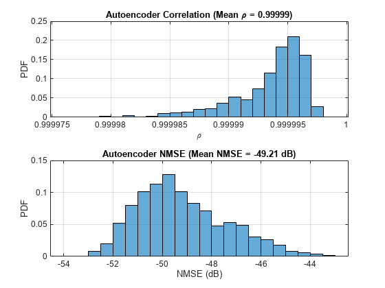
Calculate the correlation and NMSE between the input and output of the autoencoder network. The correlation is defined as

$ρ = E {\frac{1}{N} \sum_{n = 1}^{N} \frac{| {h_{}^{ˆ}}_{n}^{H} h_{n} |}{‖ {h_{}^{ˆ}}_{n} ‖_{2} ‖ h_{n} ‖_{2}}}$

where $h_{n}$ is the channel estimate at the input of the autoencoder and ${h_{}^{ˆ}}_{n}$ is the channel estimate at the output of the autoencoder. NMSE is defined as

$N M S E = E {\frac{{‖ H - H_{}^{ˆ} ‖}_{2}^{2}}{{‖ H ‖}_{2}^{2}}}$

where $H$ is the channel estimate at the input of the autoencoder and $H_{}^{ˆ}$ is the channel estimate at the output of the autoencoder.

rho = zeros(numTest,1);
nmse = zeros(numTest,1);
for n=1:numTest
    in = HTestReal(:,:,1,n) + 1i*(HTestReal(:,:,2,n));
    out = HTestRealHat(:,:,1,n) + 1i*(HTestRealHat(:,:,2,n));

    % Calculate correlation
    n1 = sqrt(sum(conj(in).*in,'all'));
    n2 = sqrt(sum(conj(out).*out,'all'));
    aa = abs(sum(conj(in).*out,'all'));
    rho(n) = aa / (n1*n2);

    % Calculate NMSE
    mse = mean(abs(in-out).^2,'all');
    nmse(n) = 10*log10(mse / mean(abs(in).^2,'all'));
end

figure
tiledlayout(2,1)
nexttile
histogram(rho,"Normalization","probability")
grid on
title(sprintf("Autoencoder Correlation (Mean \\rho = %1.5f)", ...
  mean(rho)))
xlabel("\rho"); ylabel("PDF")
nexttile
histogram(nmse,"Normalization","probability")
grid on
title(sprintf("Autoencoder NMSE (Mean NMSE = %1.2f dB)",mean(nmse)))
xlabel("NMSE (dB)"); ylabel("PDF")

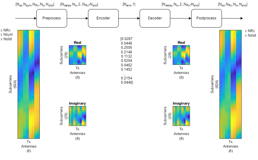
End-to-End CSI Feedback System

This figure shows the end-to-end processing of channel estimates for CSI feedback. The UE uses the CSI-RS signal to estimate the channel response for one slot, $H_{e s t}$ . The preprocessed channel estimate, $H_{t r}$ , is encoded by using the encoder portion of the autoencoder to produce a 1-by- $N_{e n c}$ compressed array. The compressed array is decompressed by the decoder portion of the autoencoder to obtain ${H_{t r}}_{}^{ˆ}$ . Postprocessing ${H_{t r}}_{}^{ˆ}$ produces ${H_{e s t}}_{}^{ˆ}$ .

End-to-end CSI compression

To obtain the encoded array, split the autoencoder into two parts: the encoder network and the decoder network.

[encNet,decNet] = helperCSINetSplitEncoderDecoder(net,"Enc_Sigmoid");
plotNetwork(net,encNet,decNet)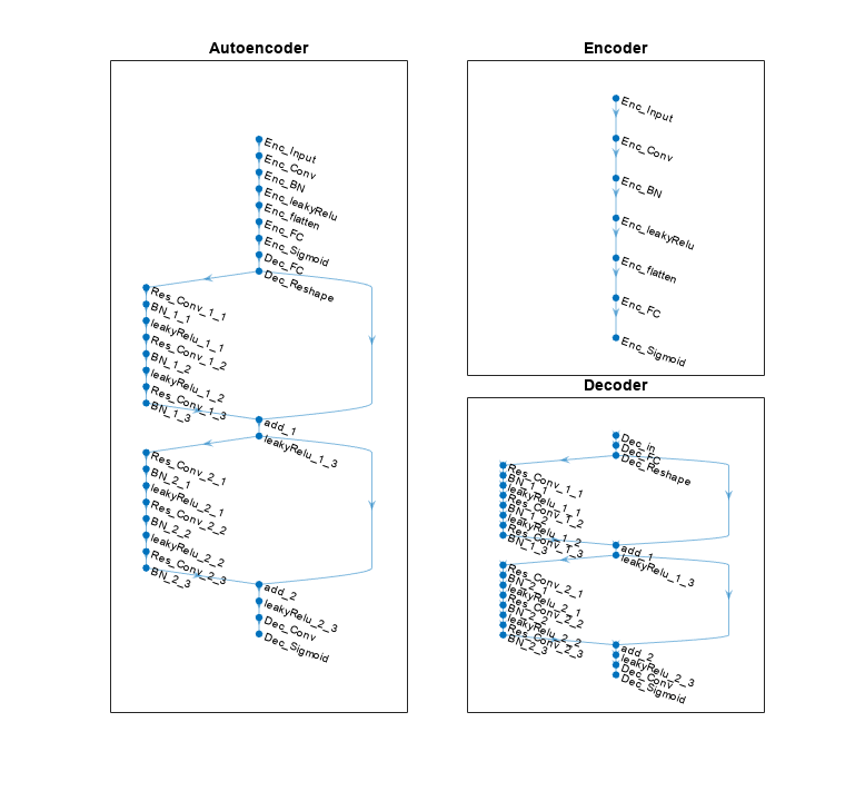

Generate channel estimates.

nSlots = 100;
Hest = helperCSINetChannelEstimate(nSlots,carrier,channel);

Encode and decode the channel estimates with Normalization set to true.

autoEncOpt.Normalization = true;
codeword = helperCSINetEncode(encNet, Hest, autoEncOpt);
Hhat = helperCSINetDecode(decNet, codeword, autoEncOpt);

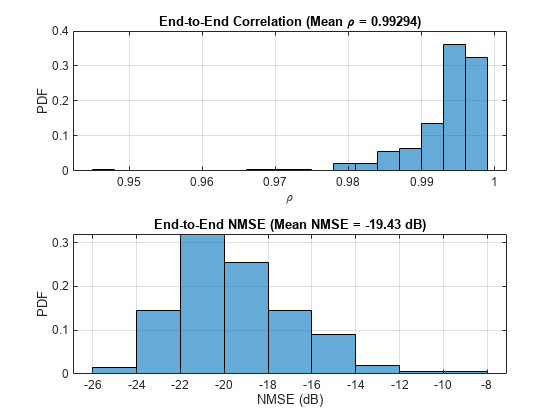
Calculate the correlation and NMSE for the end-to-end CSI feedback system.

H = squeeze(mean(Hest,2));
rhoE2E = zeros(nRx,nSlots);
nmseE2E = zeros(nRx,nSlots);
for rx=1:nRx
    for n=1:nSlots
        out = Hhat(:,rx,:,n);
        in = H(:,rx,:,n);
        rhoE2E(rx,n) = helperCSINetCorrelation(in,out);
        nmseE2E(rx,n) = helperNMSE(in,out);
    end
end
figure
tiledlayout(2,1)
nexttile
histogram(rhoE2E,"Normalization","probability")
grid on
title(sprintf("End-to-End Correlation (Mean \\rho = %1.5f)", ...
  mean(rhoE2E,'all')))
xlabel("\rho"); ylabel("PDF")
nexttile
histogram(nmseE2E,"Normalization","probability")
grid on
title(sprintf("End-to-End NMSE (Mean NMSE = %1.2f dB)", ...
  mean(nmseE2E,'all')))
xlabel("NMSE (dB)"); ylabel("PDF")

Effect of Quantized Codewords

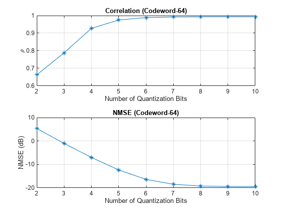
Practical systems require quantizing the encoded codeword by using a small number of bits. Simulate the effect of quantization across the range of [2, 10] bits. The results show that 6-bits is enough to closely approximate the single-precision performance.

CSI compression with autoencoder and quantization

maxVal = 1;
minVal = -1;
idxBits = 1;
nBitsVec = 2:10;
rhoQ = zeros(nRx,nSlots,length(nBitsVec));
nmseQ = zeros(nRx,nSlots,length(nBitsVec));
for numBits = nBitsVec
    disp("Running for " + numBits + " bit quantization")

    % Quantize between 0:2^n-1 to get bits
    qCodeword = uencode(double(codeword*2-1), numBits);

    % Get back the floating point, quantized numbers
    codewordRx = (single(udecode(qCodeword,numBits))+1)/2;
    Hhat = helperCSINetDecode(decNet, codewordRx, autoEncOpt);
    H = squeeze(mean(Hest,2));
    for rx=1:nRx
        for n=1:nSlots
            out = Hhat(:,rx,:,n);
            in = H(:,rx,:,n);
            rhoQ(rx,n,idxBits) = helperCSINetCorrelation(in,out);
            nmseQ(rx,n,idxBits) = helperNMSE(in,out);
        end
    end
    idxBits = idxBits + 1;
end

Running for 2 bit quantization
Running for 3 bit quantization
Running for 4 bit quantization
Running for 5 bit quantization
Running for 6 bit quantization
Running for 7 bit quantization
Running for 8 bit quantization
Running for 9 bit quantization
Running for 10 bit quantization

figure
tiledlayout(2,1)
nexttile
plot(nBitsVec,squeeze(mean(rhoQ,[1 2])),'*-')
title("Correlation (Codeword-" + size(codeword,3) + ")")
xlabel("Number of Quantization Bits"); ylabel("\rho")
grid on
nexttile
plot(nBitsVec,squeeze(mean(nmseQ,[1 2])),'*-')
title("NMSE (Codeword-" + size(codeword,3) + ")")
xlabel("Number of Quantization Bits"); ylabel("NMSE (dB)")
grid on

Further Exploration

The autoencoder is able to compress a [624 8] single-precision complex channel estimate array into a [64 1] single-precision array with a mean correlation factor of 0.99 and a NMSE of –19.55 dB. Using 6-bit quantization requires only 384 bits of CSI feedback data, which equates to a compression ratio of approximately 800:1.

display("Compression ratio is " + (624*8*32*2)/(64*6) + ":" + 1)

    "Compression ratio is 832:1"

Investigate the effect of truncationFactor on the system performance. Vary the 5G system parameters, channel parameters, and number of encoded symbols and then find the optimum values for the defined channel.

The NR PDSCH Throughput Using Channel State Information Feedback example shows how to use channel state information (CSI) feedback to adjust the physical downlink shared channel (PDSCH) parameters and measure throughput. Replace the CSI feedback algorithm with the CSI compression autoencoder and compare performance.

Helper Functions

Explore the helper functions to see the detailed implementation of the system.

Appendix: Optimize Hyperparameters with Experiment Manager

Use the Experiment Manager app to find the optimal parameters. CSITrainingProject.mlproj is a preconfigured project. Extract the project.

projectName = "CSITrainingProject";
if ~exist(projectName,"dir")
  projRoot = helperCSINetExtractProject(projectName);
else
  projRoot = fullfile(exRoot(),projectName);
end

To open the project, start the Experiment Manager app and open the following file.

disp(fullfile(".","CSITrainingProject","CSITrainingProject.prj"))

.\CSITrainingProject\CSITrainingProject.prj

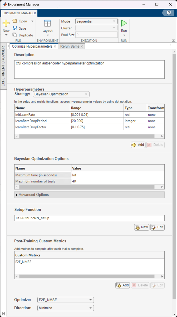
The Optimize Hyperparameters experiment uses Bayesian optimization with hyperparameter search ranges specified as in the following figure. The experiment setup function is CSIAutoEncNN_setup. The custom metric function is E2E_NMSE.

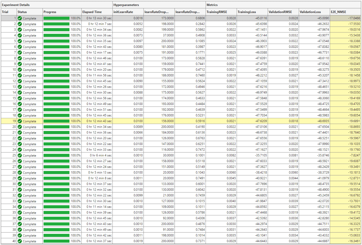
The optimal parameters are 0.01 for initial learning rate, 156 iterations for the learning rate drop period, and 0.5916 for learning rate drop factor. After finding the optimal hyperparameters, train the network with same parameters multiple times to find the best trained network.

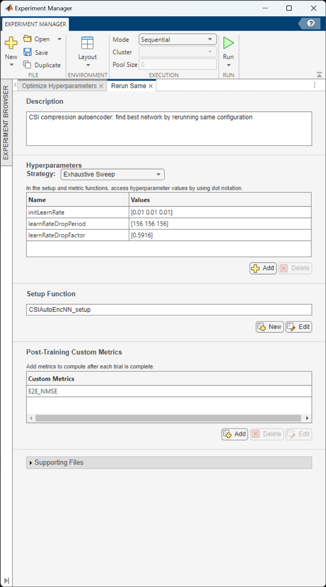
The ninth trial produced the best E2E_NMSE. This example uses this trained network as the saved network.

Configuring Batch Mode

When execution Mode is set to Batch Sequential or Batch Simultaneous, training data must be accessible to the workers in a location defined by the dataDir variable in the Prepare Data in Bulk section. Set dataDir to a network location that is accessible by the workers. For more information, see Offload Experiments as Batch Jobs to a Cluster (Deep Learning Toolbox).

Local Functions

function plotChannelResponse(Hest)
%plotChannelResponse Plot channel response

figure
tiledlayout(2,2)
nexttile
waterfall(abs(Hest(:,:,1,1))')
xlabel("Subcarriers"); 
ylabel("Symbols"); 
zlabel("Channel Magnitude")
view(15,30)
colormap("cool")
title("Rx=1, Tx=1")
nexttile
plot(squeeze(abs(Hest(:,1,:,1))))
grid on
xlabel("Subcarriers"); 
ylabel("Channel Magnitude")
legend("Rx 1", "Rx 2")
title("Symbol=1, Tx=1")
nexttile
waterfall(squeeze(abs(Hest(:,1,1,:)))')
view(-45,75)
grid on
xlabel("Subcarriers"); 
ylabel("Tx"); 
zlabel("Channel Magnitude")
title("Symbol=1, Rx=1")
nexttile
nSubCarriers = size(Hest,1);
subCarrier = randi(nSubCarriers);
plot(squeeze(abs(Hest(subCarrier,1,:,:)))')
grid on
xlabel("Tx"); 
ylabel("Channel Magnitude")
legend("Rx 1", "Rx 2")
title("Subcarrier=" + subCarrier + ", Symbol=1")
end

function valid = validateTrainingFiles(dataDir,filePrefix,expN, ...
  opt,channel,carrier)
%validateTrainingFiles Validate training data files
%   V = validateTrainingFiles(DIR,PRE,N,OPT,CH,CR) checks the DIR directory
%   for training data files with a prefix of PRE. It checks if there are
%   N*OPT.NumRxAntennas files, channel configuration is same as CH, and
%   carrier configuration is same as CR.

valid = true;
files = dir(fullfile(dataDir,filePrefix+"*"));
if isempty(files)
  valid = false;
  return
end
if exist(fullfile(dataDir,"info.mat"),"file")
  infoStr = load(fullfile(dataDir,"info.mat"));
  if ~isequal(get(infoStr.channel),get(channel)) ...
      || ~isequal(infoStr.carrier,carrier)
    valid = false;
  end
else
  valid = false;
end
if valid
  valid = (expN == (length(files)*opt.NumRxAntennas));
  % Check size of Hest in the files
  load(fullfile(files(1).folder,files(1).name),'H')
  if ~isequal(size(H),[opt.NumSubcarriers opt.NumSymbols ...
      opt.NumRxAntennas opt.NumTxAntennas])
    valid = false;
  end
end
if ~valid
  disp("Removing invalid data directory: " + files(1).folder)
  rmdir(files(1).folder,'s')
end
end

function plotNetwork(net,encNet,decNet)
%plotNetwork Plot autoencoder network
%   plotNetwork(NET,ENC,DEC) plots the full autoencoder network together
%   with encoder and decoder networks.
fig = figure;
t1 = tiledlayout(1,2,'TileSpacing','Compact');
t2 = tiledlayout(t1,1,1,'TileSpacing','Tight');
t3 = tiledlayout(t1,2,1,'TileSpacing','Tight');
t3.Layout.Tile = 2;
nexttile(t2)
plot(net)
title("Autoencoder")
nexttile(t3)
plot(encNet)
title("Encoder")
nexttile(t3)
plot(decNet)
title("Decoder")
pos = fig.Position;
pos(3) = pos(3) + 200;
pos(4) = pos(4) + 300;
pos(2) = pos(2) - 300;
fig.Position = pos;
end

function plotPreprocessingSteps(Hmean,Hdft2,Htemp,Htrunc, ...
  nSub,nTx,maxDelay)
%plotPreprocessingSteps Plot preprocessing workflow

hfig = figure;
hfig.Position(3) = hfig.Position(3)*2;
subplot(2,5,[1 6])
himg = imagesc(abs(Hmean)); 
himg.Parent.YDir = "normal"; 
himg.Parent.Position(3) = 0.05; 
himg.Parent.XTick=''; himg.Parent.YTick=''; 
xlabel(sprintf('Tx\nAntennas\n(%d)',nTx)); 
ylabel(sprintf('Subcarriers\n(%d)',nSub'));
title("Measured")
subplot(2,5,[2 7])
himg = image(abs(Hdft2)); 
himg.Parent.YDir = "normal"; 
himg.Parent.Position(3) = 0.05; 
himg.Parent.XTick=''; himg.Parent.YTick=''; 
title("2-D DFT")
xlabel(sprintf('Tx\nAngle\n(%d)',nTx)); 
ylabel(sprintf('Delay Samples\n(%d)',nSub'));
subplot(2,5,[3 8])
himg = image(abs(Htemp)); 
himg.Parent.YDir = "normal"; 
himg.Parent.Position(3) = 0.05; 
himg.Parent.Position(4) = himg.Parent.Position(4)*10*maxDelay/nSub; 
himg.Parent.Position(2) = (1 - himg.Parent.Position(4)) / 2;
himg.Parent.XTick=''; himg.Parent.YTick=''; 
xlabel(sprintf('Tx\nAngle\n(%d)',nTx)); 
ylabel(sprintf('Delay Samples\n(%d)',maxDelay'));
title("Truncated")
subplot(2,5,[4 9])
himg = imagesc(abs(Htrunc)); 
himg.Parent.YDir = "normal"; 
himg.Parent.Position(3) = 0.05; 
himg.Parent.Position(4) = himg.Parent.Position(4)*10*maxDelay/nSub; 
himg.Parent.Position(2) = (1 - himg.Parent.Position(4)) / 2;
himg.Parent.XTick=''; himg.Parent.YTick=''; 
xlabel(sprintf('Tx\nAntennas\n(%d)',nTx)); 
ylabel(sprintf('Subcarriers\n(%d)',maxDelay'));
title("2-D IDFT")
subplot(2,5,5)
himg = imagesc(real(Htrunc)); 
himg.Parent.YDir = "normal"; 
himg.Parent.Position(3) = 0.05; 
himg.Parent.Position(4) = himg.Parent.Position(4)*10*maxDelay/nSub; 
himg.Parent.Position(2) = himg.Parent.Position(2) + 0.18;
himg.Parent.XTick=''; himg.Parent.YTick=''; 
xlabel(sprintf('Tx\nAntennas\n(%d)',nTx)); 
ylabel(sprintf('Subcarriers\n(%d)',maxDelay'));
title("Real")
subplot(2,5,10)
himg = imagesc(imag(Htrunc)); 
himg.Parent.YDir = "normal"; 
himg.Parent.Position(3) = 0.05; 
himg.Parent.Position(4) = himg.Parent.Position(4)*10*maxDelay/nSub; 
himg.Parent.Position(2) = himg.Parent.Position(2) + 0.18;
himg.Parent.XTick=''; himg.Parent.YTick=''; 
xlabel(sprintf('Tx\nAntennas\n(%d)',nTx)); 
ylabel(sprintf('Subcarriers\n(%d)',maxDelay'));
title("Imaginary")
end

function rootDir = exRoot()
%exRoot Example root directory
rootDir = fileparts(which("helperCSINetDLNetwork"));
end

function loss = nmseLossdB(x,xHat)
%nmseLossdB NMSE loss in dB
in = complex(x(:,:,1,:),x(:,:,2,:));
out = complex(xHat(:,:,1,:),xHat(:,:,2,:));
nmsePerObservation = helperNMSE(in,out);
loss = mean(nmsePerObservation);
end

References

[1] Wen, Chao-Kai, Wan-Ting Shih, and Shi Jin. “Deep Learning for Massive MIMO CSI Feedback.” IEEE Wireless Communications Letters 7, no. 5 (October 2018): 748–51. https://doi.org/10.1109/LWC.2018.2818160.

[2] Zimaglia, Elisa, Daniel G. Riviello, Roberto Garello, and Roberto Fantini. “A Novel Deep Learning Approach to CSI Feedback Reporting for NR 5G Cellular Systems.” In 2020 IEEE Microwave Theory and Techniques in Wireless Communications (MTTW), 47–52. Riga, Latvia: IEEE, 2020. https://doi.org/10.1109/MTTW51045.2020.9245055.