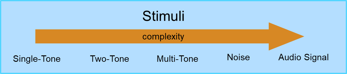
Audio Device Test Stimuli

Non-Linear System

In this example, you pass stimuli through static frequency-dependent nonlinearities defined in the supporting function, iNonlinearSystem. The function adds low-level Gaussian noise, performs a 2-band crossover filter, applies a symmetric nonlinearity to the lower crossover and a nonsymmetric nonlinearity to the upper crossover, then recombines the bands.

Single-Tone Generation

All stimuli explored in the example are built from sinusoids. Define a function to generate sinusoids assuming a 48 kHz sample rate and a required output duration of 1 second. For convenience, you analyze signals and responses in the frequency domain with a resolution equal to the number of points in the input signal. The function forces selected stimuli frequencies to fall on bins in the frequency domain to reduce spectral leakage.

fs = 48e3;
function x = iGenerateSinusoid(f,fs)
dur = 1;
fftLength = fs*dur;
binResolution = fs/fftLength;
bin = round(f/binResolution);
X = zeros(fftLength,1);
X(bin) = 1;
x = ifft(X,"symmetric");
x = x./max(abs(x));
end

Steady-State Single-Tone Signal

The single tone stimulus is simple to generate, fast, reveals harmonic distortion, the DC component, and the maximum output of fundamental compression. It is good at characterizing rub and buzz. However, it does not generate intermodulation components and is not a comprehensive assessment of nonlinear behavior.

Generate a steady-state tone at 200 Hz and then pass it through the nonlinear system. Plot the response.

The stimuli reveals that the system introduces harmonic distortion.

f = 200;

stimulus = iGenerateSinusoid(f,fs);
output = iNonlinearSystem(stimulus,fs);

iPlot(stimulus,output,fs)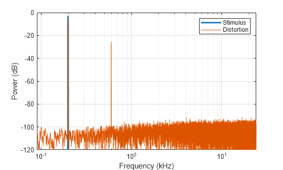

To view the total harmonic distortion of the system, use thd. The total harmonic distortion (THD) provides a single number describing the harmonic distortion resulting from a single tone input.

figure()
thd(output,fs);
xscale log
xlim([90,fs/2]/1000)
ylim([-120 0])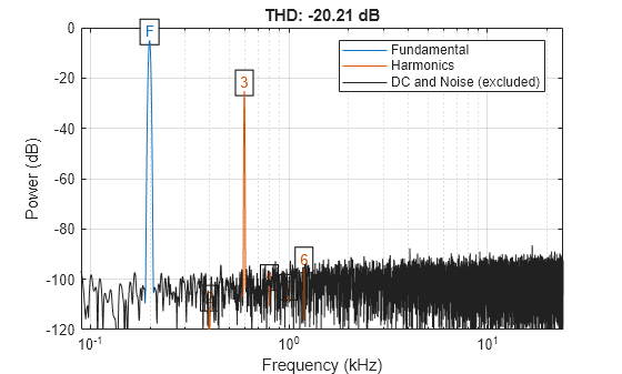

Because the lower band nonlinearity is symmetric, the harmonic distortion is odd order. Exercise the system with a 1200 Hz sinusoid. The harmonic distortion corresponding to the asymmetric nonlinearity is both odd and even ordered.

f = 1200;

stimulus = iGenerateSinusoid(f,fs);
output = iNonlinearSystem(stimulus,fs);

figure()
thd(output,fs);
xscale log
xlim([90,fs/2]/1000)
ylim([-120 0])

Stepped Single-Tone Signal

A single tone only reveals a system's response to that single tone. It is a good diagnostic tool, but to characterize a system you need to excite tones across the spectrum. Two popular options are a sweep tone and a stepped tone. A sweep, or chirp, or gliding tone, is a continuous signal whose instantaneous frequency varies logarithmically with time. A stepped tone is simply a series of steady-state tones separated by silence. Sweep tones are a more modern approach but require careful postprocessing in the analysis. See sweeptone for an example. In this example, you use a stepped single-tone to analyze the system's response across the spectrum.

Define the number of tones and range under test.

numTones = 200;
fsteps_1 = logspace(log10(10),log10(20e3),numTones);

In a loop:

No pause is required between excitations because the system under test is memory-less.

thd_tonesteps = zeros(numTones,1);
for ii = 1:numTones
    stimulus = iGenerateSinusoid(fsteps_1(ii),fs);
    output = iNonlinearSystem(stimulus,fs);
    thd_tonesteps(ii) = thd(output,fs);
end

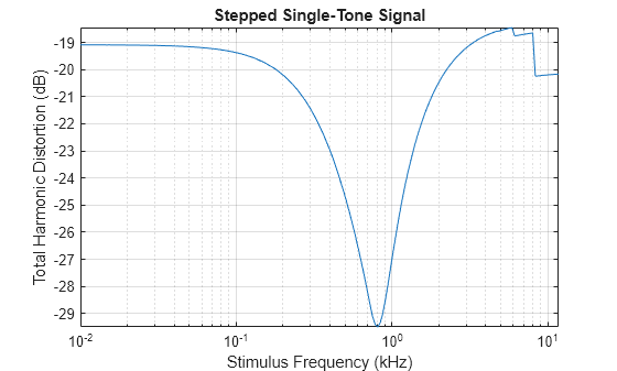
Plot the THD as a function of the stimulus frequency.

figure()
h = plot(fsteps_1/1000,thd_tonesteps);
xscale log
xlabel("Stimulus Frequency (kHz)")
ylabel("Total Harmonic Distortion (dB)")
title("Stepped Single-Tone Signal")
grid on
axis tight

Steady-State Two-Tone Signal

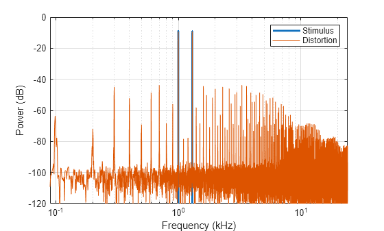
Real systems must be exercised with multiple simultaneous tones to characterize the intermodulation distortion. Generate a stimulus consisting of two tones and pass them through the system. The distortion response contains both harmonic distortion and intermodulation distortion.

Advantages of intermodulation measurement using a two-tone stimulus are that it's simple to generate, easy to separate noise and distortion, easy to interpret, good for loudspeaker diagnostics in R&D, and the stimulus and response are suitable for listening tests. Disadvantages are that the excitation tones must be carefully selected, and it does not activate the whole system.

f1 = 1000;
f2 = 1300;
stimulus = mean([iGenerateSinusoid(f1,fs),iGenerateSinusoid(f2,fs)],2);
output = iNonlinearSystem(stimulus,fs);

iPlot(stimulus,output,fs)

To characterize the intermodulation product of a two-tone stimulus, use toi. The toi function calculates the third order intercept between the harmonics and intermodulations. The third order intercept is usually the most interfering.

figure()
toi(output,fs);
xscale log
xlim([90,fs/2]./1000)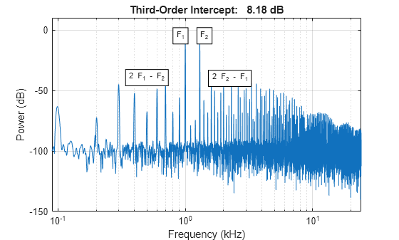

Two-Tone Step

To characterize intermodulation distortion (IMD) across the spectrum using a two-tone signal, one or both tones must sweep. Common options are to hold the bass tone and sweep the voice, hold the voice and sweep the bass, or sweep both simultaneously with either a consistent frequency difference or frequency ratio. First, you sweep the voice tone.

Define the bass frequency, range of the voice frequency, and the number of tones to test.

fs = 48e3;
f1 = 100;
t = ((0:fs-1)/fs)';
numTones = 200;
fsteps_2 = logspace(log10(500),log10(20e3),numTones);

In a loop:

toi_tonessteps = nan(numTones,1);
bassTone = iGenerateSinusoid(f1,fs);
for ii = 1:numTones
    voiceTone = iGenerateSinusoid(fsteps_2(ii),fs);
    stimulus = mean([bassTone,voiceTone],2);

    output = iNonlinearSystem(stimulus,fs);

    [~,~,~,imodpow] = toi(output,fs);

    if ~all(isnan(imodpow))
        toi_tonessteps(ii) = sum(imodpow,"omitmissing");
    end
end

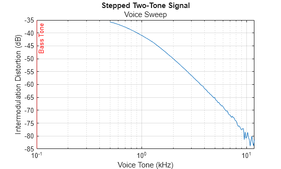
Plot the IMD as a function of the stimulus frequency. Notice that the IMD diminishes quickly as frequency increases. This is because the crossover filter in the nonlinear system diminishes the intermodulation products between the bass frequency and voice frequency.

plot(fsteps_2/1000,toi_tonessteps)
xlabel("Voice Tone (kHz)")
xscale log
ylabel("Intermodulation Distortion (dB)")
title("Stepped Two-Tone Signal","Voice Sweep")
xline(f1/1000,"r","Bass Tone")
grid on

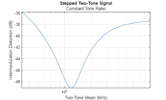
Perform a two-tone step again. This time, keep the bass and voice tone at a constant ratio.

toi_tonessteps_cntr = nan(numTones,1);
bassTone = iGenerateSinusoid(f1,fs);
toneRatio = pi;
for ii = 1:numTones
    voiceTone = iGenerateSinusoid(fsteps_2(ii),fs);
    bassTone = iGenerateSinusoid(fsteps_2(ii)/toneRatio,fs);
    stimulus = mean([bassTone,voiceTone],2);

    output = iNonlinearSystem(stimulus,fs);

    [~,~,~,imodpow] = toi(output,fs);

    if ~all(isnan(imodpow))
        toi_tonessteps_cntr(ii) = sum(imodpow,"omitmissing");
    end
end
fsteps_2_cntr = mean([fsteps_2;fsteps_2/toneRatio],1);

Plot the results. The interaction between the tones is still reduced near the crossover point. However, you can now see intermodulation products in the higher frequencies.

plot(fsteps_2_cntr/1000,toi_tonessteps_cntr)
xlabel("Two-Tone Mean (kHz)")
xscale log
axis tight
ylabel("Intermodulation Distortion (dB)")
title("Stepped Two-Tone Signal","Constant Tone Ratio")
grid on

Multi-Tone

Multi-tone stimulus excites the system in a similar way to a two-tone sweep but is significantly faster and well-suited to end-of-line testing.

The response shows both harmonic distortion and interharmonic distortion across the entire spectrum robustly--without need for careful selection of the excited frequencies. The result, "multi-tone distortion", doesn't show the generation process in detail. Multi-tone stimulus is a good tool for quality control because it is fast, it is a realistic exercise of the audio device, and it covers the entire spectrum.

Generate a multitone signal according to IEC 60268-21 [3] and pass it through the nonlinear system. Plot the stimulus and distortion.

[stimulus,xinfo] = multitone(fs);
output = iNonlinearSystem(stimulus,fs);

iPlot(stimulus,output,fs)

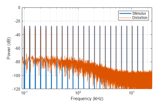
The distance between the fundamental and distortion can be evaluated in terms of perceptual masking. That is, the distance must be large enough so we do not hear it.

Because of the complex interactions of multiple forms of distortion, it is difficult to attribute distortion to particular tones, although [1] does show that the level of distortion in different parts of the spectrum can point to different aspects of a loudspeaker system.

Most commonly, the distortion results are smoothed using a sliding window as described in [2]. The smoothed result is called the multi-tone total nonlinear distortion (MTND). The MTND can be used as a fingerprint of a loudspeaker for end-of-line testing: divergence from the fingerprint warrants investigation.

Remove the fundamentals from the distortion curve, then use a simple moving average. [2] suggests several alternatives to a simple moving average but there is currently no standard best practice.

[mtnd,fvec] = iPlotMTND(stimulus,output,xinfo);

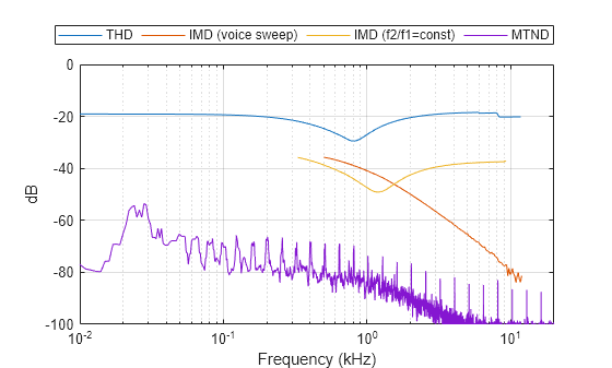
Compare the THD, IMD, and MTD results.

figure()
plot(fsteps_1/1000,thd_tonesteps, ...
    fsteps_2/1000,toi_tonessteps, ...
    fsteps_2_cntr/1000,toi_tonessteps_cntr, ...
    fvec/1000,mtnd)
grid on
xscale log
legend("THD","IMD (voice sweep)","IMD (f2/f1=const)","MTND", ...
    Location="northoutside", ...
    Orientation="horizontal")
xlabel("Frequency (kHz)")
ylabel("dB")
axis([0.01,20,-100,0])

Supporting Functions

Non-Linear System (Device Under Test)

function z = iNonlinearSystem(x,fs) 
persistent xfilt designFs
if isempty(xfilt) || ~isequal(fs,designFs)
    xfilt = crossoverFilter(1,800,SampleRate=fs,CrossoverSlopes=6);
    designFs = fs;
end
reset(xfilt) % Static Nonlinearity

% Apply nonlinearities to different frequency regions
x = x + 1e-3.*randn(size(x,1),1);
[x1,x2] = xfilt(x);
z = iSoftClip(x1) + clip(x2,-1,2/3);

z = z./max(abs(z));
end

Soft Clip

function y = iSoftClip(x)
lowerclip = x<-1;
upperclip = x>1;
middle = ~(lowerclip | upperclip);

y = x;
y(middle) = x(middle) - (x(middle).^3)/3;
y(lowerclip) = -(2/3);
y(upperclip) = (2/3);
end

Plot Multi-Tone and Smoothed Multi-Tone

function [Ysmoothed,fvec] = iPlotMTND(stimulus,response,xinfo)

[pxx,fvec] = periodogram([stimulus,response], ...
    hann(numel(stimulus),"periodic"),numel(stimulus),xinfo.SampleRate,"onesided","power");
Y = pow2db(pxx(:,2));
Y(xinfo.Tones.Bin) = nan;

Ysmoothed = movmean(Y,10,"omitmissing");

iPlot(stimulus,response,xinfo.SampleRate)
hold on
plot(fvec/1000,Ysmoothed,"k")
legend("Stimulus","Distortion","MTND")
hold off
end

Plot Response

function iPlot(stimulus,response,fs)
figure()
periodogram([stimulus,response], ...
    hann(numel(stimulus),"periodic"),numel(stimulus),fs,"onesided","power")
ph = gca;
ylim([-120,0])
xscale log
title("")
legend("Stimulus","Distortion");
ph.Children(2).LineWidth = 2;
xlim([90,fs/2]./1000)
end

References

Klippel, Wolfgang. "KLIPPEL LIVE Series 1 - Part 9: Intermodulation Distortion - Music is More than a Single Tone." YouTube video, 1:23:37. August 12, 2020. https://www.youtube.com/watch?v=XT765ItuUnI
Voishvillo, Alexander, Alexander Terekhov, Eugene Czerwinski, and Sergei Alexandrov. "Graphing, interpretation, and comparison of results of loudspeaker nonlinear distortion measurements." Journal of the Audio Engineering Society 52, no. 4 (2004): 332-357.
International Electrotechnical Commission. Sound system equipment - Part 21: Acoustical (output-based) measurements. IEC 60268-21:2018