incrementalPOD

This example shows how to use custom simulations to obtain state-snapshot data and perform POD model order reduction. By default, the POD algorithm provides three types of built-in excitation signals (chirp, impulse, and PRBS) to perform simulations. The software simulates the model and extracts state-snapshot data and approximates the controllability and observability Gramians. Alternatively, you can provide custom POD data generated from a simulation with incrementalPOD and lsim.

Generate a random state-space model with 30 states, one input, and one output and create a model order reduction task.

rng(0)
sys = rss(30,1,1);
R = reducespec(sys,"pod");

For this example, create a superimposed sinusoidal signal as an input signal for running simulations.

t = linspace(0,100,10000);
u = 0.5*(sin(1.*t)+sin(3.*t)+sin(5.*t)+sin(8.*t)+sin(10.*t));

Create incremental POD objects to store the approximation of reachability and observability Gramians.

rPOD = incrementalPOD;
oPOD = incrementalPOD;

Perform simulations of the plant model and its adjoint with the custom input signal u.

[~,~,~,~,rPOD] = lsim(sys,u,t,rPOD);
asys = adjoint(sys);
[~,~,~,~,oPOD] = lsim(asys,u,t,oPOD);

lsim generates the state-snapshot data and returns the custom POD data as output. This data is generated in a format compatible with R.Options.

Specify the custom data and run the model reduction algorithm. When you specify options CustomLr and CustomLo, the software bypasses the built in simulations and uses the data as is.

R.Options.CustomLr = rPOD;
R.Options.CustomLo = oPOD;
R = process(R);

You can now follow the typical workflow selecting the order and obtaining the reduced order model.

Obtain a reduced-order model that neglects 0.01% of the total energy.

rsys = getrom(R,MaxLoss=1e-4);
order(rsys)

ans = 
9

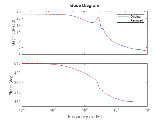
bodeplot(sys,rsys,"r--")
legend("Original","Reduced")

ans = 
  Legend (Original, Reduced) with properties:

         String: {'Original'  'Reduced'}
       Location: 'northeast'
    Orientation: 'vertical'
       FontSize: 8.1000
       Position: [0.7707 0.8532 0.1875 0.0923]
          Units: 'normalized'

  Show all properties

The reduced model provides a good approximation of the full-order model.

This example shows how to obtain a reduced-order model of a structural beam using the proper orthogonal decomposition method with custom simulation. For this example, consider a SISO sparse state-space model of a cantilever beam obtained by linearizing the structural model from the Linear Analysis of Cantilever Beam example.

Load the beam model.

load linBeam.mat
size(sys)

Sparse second-order model with 1 outputs, 1 inputs, and 3303 degrees of freedom.

For custom simulation, consider a randomly generated signal as an excitation source.

t = linspace(0,0.3,10000);
rng(0)
u = 10*rand(size(t));

Define the incremental POD object to store the POD data and run the simulation using lsim.

LrPOD = incrementalPOD;
[~,~,~,~,LrPOD] = lsim(sys,u,t,LrPOD);

For sparse state-space model, the software performs incremental POD on the fly each time a new state value becomes available. Doing so reduces the memory requirements because the state dimensions are typically very large for sparse models.

Next, create a model order reduction specification and specify the options. Because the beam model is symmetric, simulating the adjoint response and specifying data to R.Options.CustomLo are not required. Additionally, for such models you can use the Galerkin algorithm.

R = reducespec(sys,"pod");
R.Options.CustomLr = LrPOD;
R.Options.Algorithm = 'galerkin';

Run the model reduction algorithm.

R = process(R);

You can now proceed with the typical workflow selecting the order and obtaining the reduced order model.

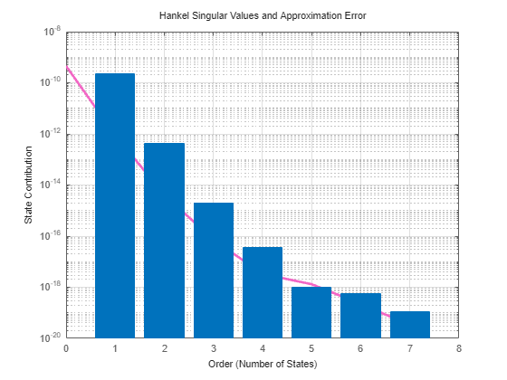
Plot the bar chart for Hankel singular values.

view(R)

Obtain the reduced order model with maximum error bound 1e-17.

rsys = getrom(R,MaxError=1e-17,Method="truncate");
order(rsys)

ans = 
8

This results in a model with order 8.

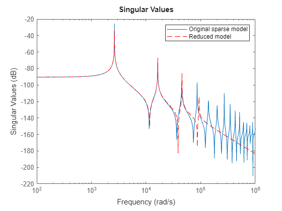
sigmaplot(sys,rsys,"r--",w)
legend("Original sparse model","Reduced model");

The reduced-order model captures the first three dominant modes of the beam accurately.

This example shows how create an incremental proper orthogonal decomposition (POD) and analyze the snapshot data stored in the object. An incrementalPOD object computes a low-rank approximation $\mathit{X}={\mathit{URV}}^{\mathit{T}}$ of the snapshot matrix $\mathit{X}$.

To start an incremental POD, initialize the object.

xPOD1 = incrementalPOD;

In POD-based model reduction, you provide the snapshots of state data. To generate state data, you typically run custom simulations with lsim. The lsim function also supports populating the xPOD object directly during the simulation. Create a random state-space and run a simulation to update the POD object.

rng(0)
sys = rss(10,1,1);
xinit = randn(10,1);
t1 = 0:0.02:5;  
u1 = randn(1,numel(t1));
[~,~,~,~,xPOD1] = lsim(sys,u1,t1,xinit,xPOD1)

xPOD1 = 
  incrementalPOD with properties:

    Snapshots: 251
      MaxRank: 10
      RankTol: 1.0000e-06
    Transform: []

lsim generates the state data and the incrementalPOD object performs on-the-fly POD by updating the URV decomposition for each simulation step.

You can also run more simulations to enrich the incremental POD with more data. As the new data becomes available, the object updates the URV approximation.

xPOD2 = incrementalPOD;
t2 = 5:0.02:8;  
u2 = randn(1,numel(t2));
[~,~,~,~,xPOD2] = lsim(sys,u2,t2,xinit,xPOD2)

xPOD2 = 
  incrementalPOD with properties:

    Snapshots: 151
      MaxRank: 10
      RankTol: 1.0000e-06
    Transform: []

You can combine multiple incremental PODs of state data from different simulations of a model. The state data must be of compatible sizes.

xPODm = merge(xPOD1,xPOD2)

xPODm = 
  incrementalPOD with properties:

    Snapshots: 402
      MaxRank: 10
      RankTol: 1.0000e-06
    Transform: []

Merging these two PODs is equivalent to running sequential simulations on the same POD object.

xPOD = incrementalPOD;
[~,~,~,~,xPOD] = lsim(sys,u1,t1,xinit,xPOD);
[~,~,~,~,xPOD] = lsim(sys,u2,t2,xinit,xPOD)

xPOD = 
  incrementalPOD with properties:

    Snapshots: 402
      MaxRank: 10
      RankTol: 1.0000e-06
    Transform: []

Compute a truncated SVD of ${\mathit{XX}}^{\mathit{T}}$, use the svd function.

[Ur,Sr] = svd(xPODm);
[Ur2,Sr2] = svd(xPOD);

This provides the approximation ${\mathit{XX}}^{\mathit{T}}\approx {\mathit{U}}_{\mathit{r}}{\Sigma }_{\mathit{r}}{\mathit{U}}_{\mathit{r}}^{\mathit{T}}$. Here, $\mathit{X}$ is the state snapshot data processed by incremental proper orthogonal decomposition (POD), ${\Sigma }_{\mathit{r}}$ matrix contains the dominant singular values, and columns of ${\mathit{U}}_{\mathit{r}}$ are the corresponding dominant left singular vectors.

XXt = Ur*diag(Sr.^2)*Ur';
XXt2 = Ur2*diag(Sr2.^2)*Ur2';
norm(XXt-XXt2,"fro")

ans = 
1.9016e-14

You can see that sequential simulations with the same POD or merging two PODs is equivalent.

This example shows how to use the state data collected during model simulation in Simulink® with proper orthogonal decomposition model order reduction.

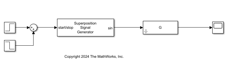
This examples uses a model that simulates a plant G of order 48 to a superimposed sinusoidal perturbation signal and collects the state data of the plant. To generate the perturbation signal, the model uses a Superposition Signal Generator block from Simulink® Control Design™ software. In this model, the block generates the sinusoidal signal at 100 frequency points between 1 rad/s and 1000 rad/s.

Open the model.

load building.mat G
w = logspace(1,3,100);
mdl = "podSimModel";
open_system(mdl)

To store the state-snapshot data for input-to-state and output-to-state maps, simulate the model and its adjoint.

set_param("podSimModel/LTI System","sys","G")
set_param(mdl,"StateSaveName","statesSimLr")
sim(mdl);
aG = adjoint(G);
set_param("podSimModel/LTI System","sys","aG")
set_param(mdl,"StateSaveName","statesSimLo")
sim(mdl);

Create incremental POD objects to store the approximation of reachability and observability Gramians.

LrPOD = incrementalPOD; 
LoPOD = incrementalPOD;

Then, to apply incremental POD to the collected state data, you can use the update function

LrPOD = update(LrPOD,statesSimLr{1}.Values.Data');
LoPOD = update(LoPOD,statesSimLo{1}.Values.Data');

Now, you can create the model order reduction specification for this plant and specify the custom data options. When you specify options CustomLr and CustomLo, the software bypasses the built in simulations and uses the data as is.

R = reducespec(G,"pod");
R.Options.CustomLr = LrPOD;
R.Options.CustomLo = LoPOD;

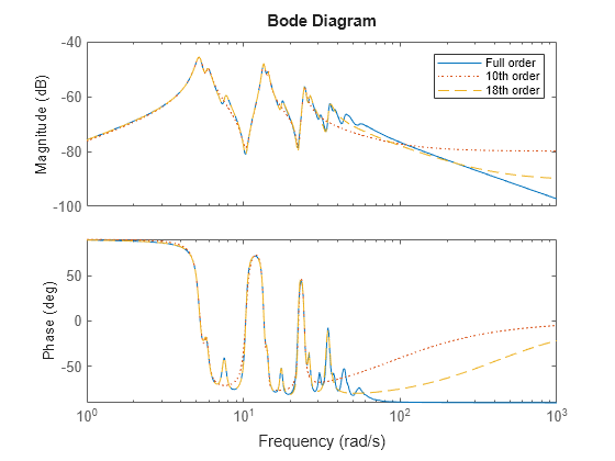
Obtain the reduced models with orders 10 and 18 and compare the Bode response with original model.

rsys = getrom(R,Order=[10,18]);
bodeplot(G,rsys(:,:,1),":",rsys(:,:,2),"--",logspace(0,3,500))
legend("Full order","10th order","18th order");

Both models provide a good approximation in the low frequency range. The 18th-order model provides a much better approximation overall.