ProperOrthogonalDecomposition

This example shows how to create a model order reduction specification for a LTI model using the proper orthogonal decomposition (POD) method.

For this example, generate a random discrete-time state-space model with 40 states.

rng(0)
sys = drss(40);

To create a specification object, use the reducespec function.

R = reducespec(sys,"pod")

R = 
  ProperOrthogonalDecomposition with properties:

      Sigma: []
      Error: []
     Energy: []
       Loss: []
         Lr: []
         Lo: []
    Options: [1×1 mor.ProperOrthogonalDecompositionOptions]

Notice that reducespec does not perform any computation and creates only the object. This allows you to set additional options before running the model order reduction algorithm, such as pseudorandom binary sequence as an excitation signal for POD simulations.

R.Options.Excitation = "prbs";

For POD, you can visualize the contributions in terms of the principal singular values, normalized energies, or neglected fraction of total energy. By default, the view function plots the principal singular values.

view(R)

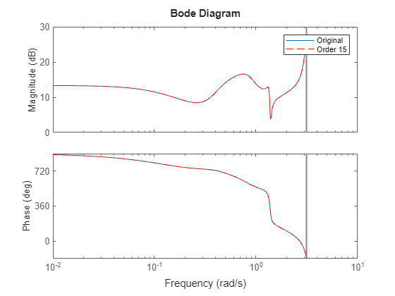
For this example, select an order of 15 since it is the first order with an approximate error less than 1e-4. In general, you can select the order explicitly or based on the desired absolute or relative approximation errors. Compute the reduced-order model.

rsys = getrom(R,Order=15);

Plot the Bode response of both models.

figure
bodeplot(sys,rsys,"r--")
legend("Original","Order 15")

ans = 
  Legend (Original, Order 15) with properties:

         String: {'Original'  'Order 15'}
       Location: 'northeast'
    Orientation: 'vertical'
       FontSize: 8.1000
       Position: [0.7727 0.8532 0.1855 0.0923]
          Units: 'normalized'

  Show all properties

Reduced-order model provides a good approximation of the original model.

This example shows how to reduce a sparse structural model using Proper Orthogonal Decomposition.

Load the model data.

load skyScraperModel.mat
size(sys)

Sparse second-order model with 1 outputs, 1 inputs, and 15439 degrees of freedom.

w = logspace(-2,4,250);
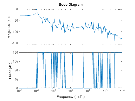
bodeplot(sys,w)

The model is undamped and has a highly resonant frequency response. Use POD to reduce the model order.

R = reducespec(sys,"pod");

Specify the frequency range of focus and excitation signal. Typically, for undamped models, you may also need to increase the number of simulation steps to get a more accurate response.

R.Options.Focus = [1e-2 1];
R.Options.Excitation = "chirp";
R.Options.NumStep = 300;

Run the model reduction algorithm and store the data in the specification.

R = process(R);

Simulating the model's response...
   Completed simulation 1 of 1.

Because this model is symmetric, the software runs a single simulation to obtain input-to-dof mapping.

Obtain the reduced-order model that neglects 1e-6 fraction of total energy.

rsys = getrom(R,MaxLoss=1e-6,Method="truncate");
size(rsys)

State-space model with 1 outputs, 1 inputs, and 54 states.

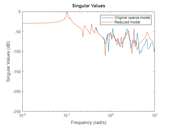
This results in a reduced model of order 54.

Compare the response of the two models.

sigmaplot(sys,rsys,w);
legend("Original sparse model","Reduced model");
xlim([1e-2 10])

This example shows how to use custom simulations to obtain state-snapshot data and perform POD model order reduction. By default, the POD algorithm provides three types of built-in excitation signals (chirp, impulse, and PRBS) to perform simulations. The software simulates the model and extracts state-snapshot data and approximates the controllability and observability Gramians. Alternatively, you can provide custom POD data generated from a simulation with incrementalPOD and lsim.

Generate a random state-space model with 30 states, one input, and one output and create a model order reduction task.

rng(0)
sys = rss(30,1,1);
R = reducespec(sys,"pod");

For this example, create a superimposed sinusoidal signal as an input signal for running simulations.

t = linspace(0,100,10000);
u = 0.5*(sin(1.*t)+sin(3.*t)+sin(5.*t)+sin(8.*t)+sin(10.*t));

Create incremental POD objects to store the approximation of reachability and observability Gramians.

rPOD = incrementalPOD;
oPOD = incrementalPOD;

Perform simulations of the plant model and its adjoint with the custom input signal u.

[~,~,~,~,rPOD] = lsim(sys,u,t,rPOD);
asys = adjoint(sys);
[~,~,~,~,oPOD] = lsim(asys,u,t,oPOD);

lsim generates the state-snapshot data and returns the custom POD data as output. This data is generated in a format compatible with R.Options.

Specify the custom data and run the model reduction algorithm. When you specify options CustomLr and CustomLo, the software bypasses the built in simulations and uses the data as is.

R.Options.CustomLr = rPOD;
R.Options.CustomLo = oPOD;
R = process(R);

You can now follow the typical workflow selecting the order and obtaining the reduced order model.

Obtain a reduced-order model that neglects 0.01% of the total energy.

rsys = getrom(R,MaxLoss=1e-4);
order(rsys)

ans = 
9

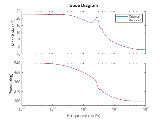
bodeplot(sys,rsys,"r--")
legend("Original","Reduced")

ans = 
  Legend (Original, Reduced) with properties:

         String: {'Original'  'Reduced'}
       Location: 'northeast'
    Orientation: 'vertical'
       FontSize: 8.1000
       Position: [0.7707 0.8532 0.1875 0.0923]
          Units: 'normalized'

  Show all properties

The reduced model provides a good approximation of the full-order model.

This example shows how to obtain a reduced-order model of a structural beam using the proper orthogonal decomposition method with custom simulation. For this example, consider a SISO sparse state-space model of a cantilever beam obtained by linearizing the structural model from the Linear Analysis of Cantilever Beam example.

Load the beam model.

load linBeam.mat
size(sys)

Sparse second-order model with 1 outputs, 1 inputs, and 3303 degrees of freedom.

For custom simulation, consider a randomly generated signal as an excitation source.

t = linspace(0,0.3,10000);
rng(0)
u = 10*rand(size(t));

Define the incremental POD object to store the POD data and run the simulation using lsim.

LrPOD = incrementalPOD;
[~,~,~,~,LrPOD] = lsim(sys,u,t,LrPOD);

For sparse state-space model, the software performs incremental POD on the fly each time a new state value becomes available. Doing so reduces the memory requirements because the state dimensions are typically very large for sparse models.

Next, create a model order reduction specification and specify the options. Because the beam model is symmetric, simulating the adjoint response and specifying data to R.Options.CustomLo are not required. Additionally, for such models you can use the Galerkin algorithm.

R = reducespec(sys,"pod");
R.Options.CustomLr = LrPOD;
R.Options.Algorithm = 'galerkin';

Run the model reduction algorithm.

R = process(R);

You can now proceed with the typical workflow selecting the order and obtaining the reduced order model.

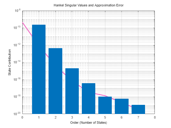
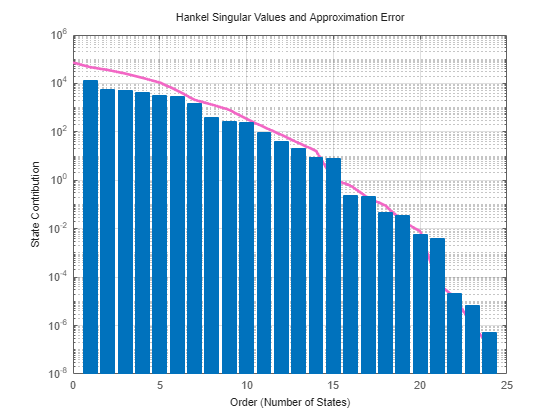
Plot the bar chart for Hankel singular values.

view(R)

Obtain the reduced order model with maximum error bound 1e-17.

rsys = getrom(R,MaxError=1e-17,Method="truncate");
order(rsys)

ans = 
8

This results in a model with order 8.

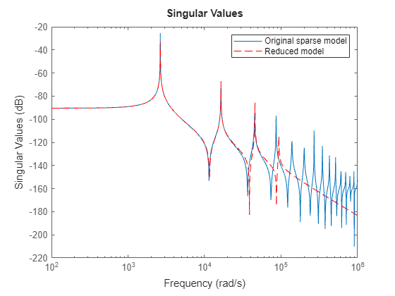
sigmaplot(sys,rsys,"r--",w)
legend("Original sparse model","Reduced model");

The reduced-order model captures the first three dominant modes of the beam accurately.

This example shows how to reduce models with large number of inputs or outputs using the proper orthogonal decomposition algorithm. For this example, consider a a three-story building model described in the Active Vibration Control in Three-Story Building example. The model has 20 outputs, 2 inputs, and 30 states. Since POD is a simulation-based technique, reducing models with a large number of inputs and output can be inefficient.

Load the model data.

load threeStoryBuilding.mat
size(PF)

State-space model with 20 outputs, 2 inputs, and 30 states.

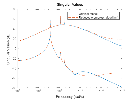
Since this is a model with many outputs and just two inputs, one way to avoid running several simulations is to use the Compress algorithm. The Compress algorithm is an acceleration of Balanced for tall or wide models (few inputs, many outputs or few outputs, many inputs). The algorithm runs the cheapest simulation (input-to-state if few inputs), uses the resulting POD of state-snapshots to compress the output and find the dominant output directions, and then performs the adjoint simulation with this reduced output.

Create the model order reduction specification and specify the options.

R = reducespec(PF,"POD");
R.Options.Algorithm = "compress";
R.Options.Excitation = "prbs";

Obtain the reducer-order model that neglects 1% of the total energy. This results in a 15th-order model.

rsys = getrom(R,MaxLoss=1e-3);
size(rsys)

State-space model with 20 outputs, 2 inputs, and 15 states.

sigmaplot(PF,rsys,"--")
legend("Original model","Reduced (compress algorithm)");

Alternatively, you can use input and and output weights to reduce I/O dimension if you know the critical or dominant inputs and outputs through physical insights.

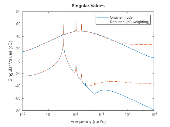
For this model, select the outputs 13, 14, 15 which correspond to the inter-story drift in the building, and emphasize input 1 which is the ground acceleration during an earthquake. Create a model reduction specification, specify the weights, and set the options.

Wy = zeros(3,20);
Wy(:,13:15) = eye(3);
Wu = [1e3;1];
R1 = reducespec(PF,"POD");
R1.Options.Focus = [1,1e3];
R1.Options.InputWeight = Wu;
R1.Options.OutputWeight = Wy;
R1.Options.Excitation = "prbs";

Obtain a reduced model of order 15.

rsys1 = getrom(R1,Order=15);
size(rsys1)

State-space model with 20 outputs, 2 inputs, and 15 states.

Compare the frequency response of the models.

sigmaplot(PF,rsys1,"--")
legend("Original model","Reduced (I/O weighting)");

The emphasized input-output channels contribute to the majority of system dynamics and the reduced model provides a good approximation of the original model.

References

[1] Pinnau, René. “Model Reduction via Proper Orthogonal Decomposition.” In Model Order Reduction: Theory, Research Aspects and Applications, edited by Wilhelmus H. A. Schilders, Henk A. van der Vorst, and Joost Rommes, 95–109. Berlin, Heidelberg: Springer, 2008. https://doi.org/10.1007/978-3-540-78841-6_5.
[2] Liang, Y.C., H.P. Lee, S.P. Lim, W.Z. Lin, K.H. Lee, and C.G. Wu. “PROPER ORTHOGONAL DECOMPOSITION AND ITS APPLICATIONS—PART I: THEORY.” Journal of Sound and Vibration 252, no. 3 (May 2002): 527–44. https://doi.org/10.1006/jsvi.2001.4041.
[3] Willcox, K., and J. Peraire. “Balanced Model Reduction via the Proper Orthogonal Decomposition.” AIAA Journal 40, no. 11 (November 2002): 2323–30. https://doi.org/10.2514/2.1570.
[4] Rowley, C. W. “MODEL REDUCTION FOR FLUIDS, USING BALANCED PROPER ORTHOGONAL DECOMPOSITION.” International Journal of Bifurcation and Chaos 15, no. 03 (March 2005): 997–1013. https://doi.org/10.1142/S0218127405012429.
[5] Moore, B. “Principal Component Analysis in Linear Systems: Controllability, Observability, and Model Reduction.” IEEE Transactions on Automatic Control 26, no. 1 (February 1981): 17–32. https://doi.org/10.1109/TAC.1981.1102568.
[6] Reis, Timo, and Tatjana Stykel. “Balanced Truncation Model Reduction of Second-Order Systems.” Mathematical and Computer Modelling of Dynamical Systems 14, no. 5 (October 2008): 391–406. https://doi.org/10.1080/13873950701844170.
Version History
Introduced in R2024b