LPV Approximation of Boost Converter Model

Boost Converter Model

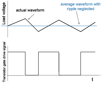
A Boost Converter circuit converts a DC voltage to another DC voltage by controlled chopping or switching of the source voltage. The request for a certain load voltage is translated into a corresponding requirement for the transistor duty cycle. The duty cycle modulation is typically several orders of magnitude slower than the switching frequency, which produces an average voltage with relatively small ripples.

In practice, disturbances in the source voltage and the resistive load also affect the actual load voltage.

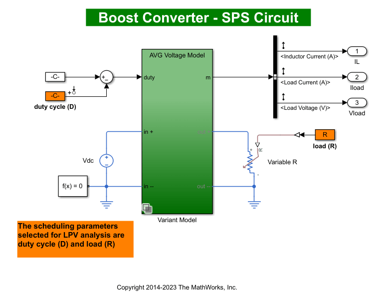
Open the Simulink® model.

mdl = 'BoostConverterExampleModel';
open_system(mdl)

The circuit in the model is characterized by high-frequency switching. The model uses a sample time of 25 ns. The Boost Converter block used in the model is a variant subsystem that implements two different versions of the converter dynamics. The model takes the duty cycle value as its only input and produces three outputs: inductor current, load current, and load voltage.

Due to the high-frequency switching and short sample time, the model simulates slowly.

Batch Trimming and Linearization

In many applications, the average voltage delivered in response to a certain duty cycle profile is of interest. Such behavior is studied at time scales several decades larger than the fundamental sample time of the circuit. These average models for the circuit are derived by analytical considerations based on averaging of power dynamics over certain time periods. The BoostConverterExampleModel model implements such an average model of the circuit as its first variant, the AVG Voltage Model variant. This variant typically executes faster than the Low Level Model variant.

The average model is not a linear system. It shows nonlinear dependence on the duty cycle and the load variations. To produce a faster simulation and to help with voltage stabilizing controller design, you can linearize the model at various duty cycle and load values. For this example, use the snapshot-based trimming and linearization. The scheduling parameters are the duty cycle d and resistive load R. You trim and linearize the model for several values of the scheduling parameters.

Select a span of 10%–60% for the duty cycle variation and a span of 4–15 ohms for the load variation. Select five values in these ranges for each scheduling variable and make a grid of all possible combinations of their values.

nD = 5;
nR = 5;
dspace = linspace(0.1,0.6,nD); % Values of d in 10%-60% range
Rspace = linspace(4,15,nR);    % Values of Rin 4-15 Ohms range
[dgrid,Rgrid] = ndgrid(dspace,Rspace);  % All combinations of d and R values

Create a parameter structure array for the scheduling parameters.

params(1).Name = 'd';
params(1).Value = dgrid;
params(2).Name = 'R';
params(2).Value = Rgrid;

A simulation of the model under various conditions shows that the model outputs settle down to their steady-state values before 0.01 s. Therefore, use t = 0.01 s as the snapshot time. Compute equilibrium operating points at the snapshot time using the findop function. This operation takes several minutes to finish.

op = findop(mdl,0.01,params);

To linearize the model, first obtain the linearization input and output points from the model.

io = getlinio(mdl);

Configure the linearization options to store linearization offsets.

opt = linearizeOptions('StoreOffsets', true);

Linearize the model at the operating points in array op.

[linsys,~,info] = linearize(mdl,op,io,params,opt);

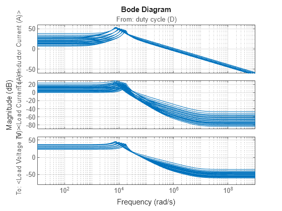
Plot the linear system array.

bodemag(linsys)
grid on

LPV Model

Use ssInterpolant to create an LPV model that interpolates the linearized models and offsets over the ($\mathit{d}$,$\mathit{R}$) operating range.

lpvsys = ssInterpolant(linsys,info.Offsets);

LPV Simulation

To simulate the model, use an input profile for the duty cycle that roughly covers its scheduling range. Also, vary the resistive load to simulate load disturbances. Generate the duty cycle profile din.

t = linspace(0,.05,1e3)';
din = 0.25*sin(2*pi*t*100)+0.25;
din(500:end) = din(500:end)+.1;

Generate the resistive load profile rin.

rin = linspace(4,12,length(t))';
rin(500:end) = rin(500:end)+3;
rin(100:200) = 6.6;

Plot the scheduling parameter profiles.

clf
yyaxis left
plot(t,din)
xlabel('Time (s)')
ylabel('Duty Cycle')
yyaxis right
plot(t,rin)
ylabel('Resistive Load (Ohm)')
title('Scheduling Parameter Profiles for Simulation')

Use lsim to simulate the response of the LPV approximation to this stimulus.

p = [din rin];  % scheduling variables
xinit = info.Offsets(1).x;
y = lsim(lpvsys,din,t,xinit,p);

Simulate the boost converter LPV model implemented using the LPV System block and plot the results.

% Offset data for LPV block
offsets = getOffsetsForLPV(info);
yoff = offsets.y;
xoff = offsets.x;
uoff = offsets.u;
simOut = sim('BoostConverterLPVModel','StopTime','0.05');
lpvBlockSim = simOut.logsout.getElement('ysim');
tsim = lpvBlockSim.Values.Time;
ysim = lpvBlockSim.Values.Data(:,:);
clf
subplot(311)
plot(t,y(:,1),tsim,ysim(:,1))
ylabel(lpvsys.OutputName{1});
subplot(312)
plot(t,y(:,2),tsim,ysim(:,2))
ylabel(lpvsys.OutputName{2});
subplot(313)
plot(t,y(:,3),tsim,ysim(:,3))
ylabel(lpvsys.OutputName{3});
legend('LPV object simulation','LPV system block simulation','location','best')

These results match the simulation results obtained with the LPV System block.

Discretization of LPV Model

Compute an equivalent discretized LPV model of the boost converter. Discretization facilitates fixed-step simulation and code generation for this model. Compare the results with those of the continuous model.

dlpvsys = c2d(lpvsys,t(2)-t(1),'tustin');
yd = lsim(dlpvsys,din,t,xinit,p);
clf
subplot(311)
plot(t,y(:,1),t,yd(:,1),'--')
ylabel(lpvsys.OutputName{1});
subplot(312)
plot(t,y(:,2),t,yd(:,2),'--')
ylabel(lpvsys.OutputName{2});
subplot(313)
plot(t,y(:,3),t,yd(:,3),'--')
ylabel(lpvsys.OutputName{3});
legend('Continuous','Discrete','location','best')

Close the model.

close_system(mdl,0)