Main Content

ssInterpolant

Build gridded LTV or LPV model from state-space data

Since R2023a

Description

For a collection of local ss models sampled in time or parameter space, ssInterpolant builds a linear time-varying (LTV) or linear parameter-varying (LPV) model that interpolates local LTI behaviors into global LTV or LPV behavior. You can also use ssInterpolant to turn analytic LTV or LPV models into gridded LTV or LPV models, or to resample gridded LTV or LPV models.

sys = ssInterpolant(ssArray) constructs the LTV or LPV interpolant from the array of state-space models ssArray. For this array, the ssArray.SamplingGrid property specified the underlying time or parameter grid, which can be rectangular or consist of scattered samples, and ssArray.Offsets specifies the linearization offsets. (since R2024a)

example

sys = ssInterpolant(ssArray,offsets) explicitly specifies the offsets as a structure array offsets containing the derivative, state, input, and output linearization offsets. This syntax is equivalent to:

ssArray.Offsets = offsets;
vsys = ssInterpolant(ssArray);

example

sys = ssInterpolant(vSys,S) constructs the interpolant by sampling an existing LTV or LPV model vSys at a grid of time and parameter values specified in S.

example

sys = ssInterpolant(___,IMethod,EMethod) specifies both the interpolation and extrapolation methods. You can specify these methods as the last input arguments in any of the previous syntaxes.

example

Examples

collapse all

This example shows how to create an LPV model from an array of state space models and associated offsets obtained from batch linearization of a water-tank Simulink® model.

Open the Simulink model.

mdl = 'watertankNLModel';
open_system(mdl)

Specify the initial condition for water height.

h0 = 10;

Specify model linear analysis points.

io(1) = linio('watertankNLModel/Step',1,'input');
io(2) = linio('watertankNLModel/H',1,'output');

Simulate the model and extract operating points at time snapshots.

tlin = [0 30 40 50 60 70 80];
op = findop(mdl,tlin);

Compute the linearizations along with offsets.

options = linearizeOptions('StoreOffsets',true);
[linsys,~,info] = linearize(mdl,io,op,options);

Specify a grid of height values and construct the LPV model. For this model, height is the first state.

h = zeros(size(tlin));
for ct=1:numel(h)
   h(ct) = op(ct).States(1).x;
end
linsys.SamplingGrid.H = h;
linsys.Offsets = info.Offsets;
gLPV = ssInterpolant(linsys,'spline')
Continuous-time state-space LPV model with 1 outputs, 1 inputs, 1 states, and 1 parameters.

Simulate the watertank model.

h0 = 15;
sim(mdl);
usim = getElement(logsOut,'V');
hsim = getElement(logsOut,'H');

Simulate the LPV model with the exact parameter trajectory.

t = linspace(0,150,200);
p = @(t,x,u) x(1);
u = interp1(usim.Values.Time,usim.Values.Data,t);
ylpv = lsim(gLPV,u,t,h0,p);

Plot the results.

plot(hsim.Values.Time,hsim.Values.Data,t,ylpv,'--')
legend('Simulink model','LPV model')

Figure contains an axes object. The axes object contains 2 objects of type line. These objects represent Simulink model, LPV model.

The LPV model provides a good approximation of the nonlinear model.

For this example, dataFcnMaglev.m defines the matrices and offsets of a magnetic levitation system. The magnetic levitation controls the height of a levitating ball using a coil current that creates a magnetic force on the ball.

Create an LPV model.

h0 = 1;
lpvSys = lpvss('h',@dataFcnMaglev,0,0,h0)
Continuous-time state-space LPV model with 1 outputs, 1 inputs, 2 states, and 1 parameters.
lpvSys.StateName = {'h','hdot'};
lpvSys.InputName = 'current';
lpvSys.InputName = 'height';

Define parameter variation for height h.

hmin = 0.05;
hmax = 0.25;
hcd = linspace(hmin,hmax,5);
SamplingGrid.h = hcd;

Convert to a gridded model.

glpvSys1 = ssInterpolant(lpvSys,SamplingGrid)
Continuous-time state-space LPV model with 1 outputs, 1 inputs, 2 states, and 1 parameters.

This command is equivalent to constructing a gridded model from an array of local models sampled at the same parameter space.

ssArray = psample(lpvSys,SamplingGrid);
glpvSys2 = ssInterpolant(ssArray);

For this example consider an array of state space models and associated offsets obtained from batch linearization of a water-tank Simulink® model in the Create LPV Model from Batch Linearization Results example.

The dynamics of this water-tank system are described by this equation.

AdHdt=bV-aH

Load the linearization results.

load watertankLinModel.mat

Construct a gridded model with the spline interpolation method and clip extrapolation method.

glpv1 = ssInterpolant(linsys,info.Offsets,"spline","clip");

Construct a gridded model with the spline extrapolation.

glpv2 = ssInterpolant(linsys,info.Offsets,"spline","spline");

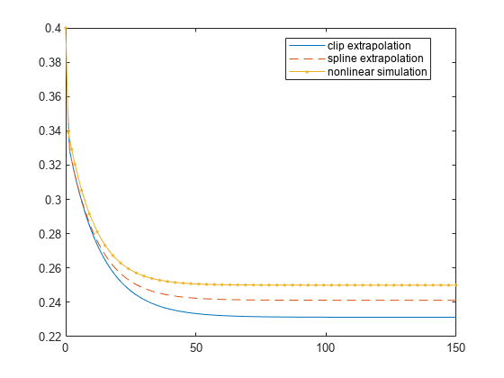
Compare simulation results of both gridded models when the initial height starts from a point outside the constructing grid. Set the height such that the tank is almost empty.

h0 = 0.4; 
sim("watertankNLModel.slx");
usim = getElement(logsOut,"V");
hsim = getElement(logsOut,"H");

Simulate the LPV models with the exact parameter trajectory.

t = linspace(0,150,200);
p = @(t,x,u) x(1);
u = interp1(usim.Values.Time,usim.Values.Data,t);
ylpv1 = lsim(glpv1,u,t,h0,p);
ylpv2 = lsim(glpv2,u,t,h0,p);
plot(t,ylpv1,t,ylpv2,"--",hsim.Values.Time,hsim.Values.Data,".-")
legend("clip extrapolation","spline extrapolation", ...
    "nonlinear simulation",Location="best")

Figure contains an axes object. The axes object contains 3 objects of type line. These objects represent clip extrapolation, spline extrapolation, nonlinear simulation.

When the tank is almost empty, the spline method captures the rapid slope change resulting from the nonlinearity better than the clip method.

Input Arguments

collapse all

Array of state-space (ss) models. Use the SamplingGrid property of the state-space object to specify the time and parameter dependence of the models in ssArray, and assign time and parameter values to each model. The field names of SamplingGrid become the parameters of the LPV model, except for the field Time which is interpreted as describing the time dependence. If Time is the only field, ssInterpolant returns an LTV model. The function ignores fields with constant value.

Additionally, you can use the Offsets property of ssArray to specify the derivative, state, input, and output linearization offsets (since R2024a). See ss reference page for more information on the SamplingGrid and Offsets properties.

You can also obtain ssArray and corresponding offsets in one of the following ways:

  • Perform batch linearization of a Simulink® model with StoreOffsets option. For more information, see linearize (Simulink Control Design) and linearizeOptions (Simulink Control Design).

  • Sample an existing LTV or LPV model. For more information, see sample.

Model offsets, specified as a structure array with the same dimensions as ssArray. Each offset structure must have the following fields:

FieldDescription
xState offsets, specified as a column vector of length nx, where nx is the number of states in ssArray
dxDerivative offsets, specified as a column vector of length nx, where nx is the number of states in ssArray
uInput offsets, specified as a column vector of length nu, where nu is the number of inputs in ssArray
yOutput offsets, specified as a column vector of length ny, where ny is the number of outputs in ssArray

You can also obtain ssArray and corresponding offsets in one of the following ways:

  • Perform batch linearization of a Simulink model with StoreOffsets option. For more information, see linearize (Simulink Control Design) and linearizeOptions (Simulink Control Design).

  • Sample an existing LTV or LPV model. For more information, see sample.

You can also set any of the fields to [] when the model has no offsets.

LTV or LPV model, specified as an ltvss or lpvss object.

If vSys is an ltvss or lpvss object, ssInterpolant builds a gridded LTV or LPV model at the grid values specified using S.

Sampling grid values, specified as a structure. S defines a grid of time and/or parameter values where vSys is sampled. The gridded LTV or LPV model interpolates between these grid points.

  • For LTV models, S is a structure array with field Time. For example, if an array Tvalues specifies the sampling time, S is the following structure.

    S = struct('Time',Tvalues)
  • For LPV models, S is a structure with fields for parameter names corresponding to the ParameterName property of the LPV model vSys, and Time. For example, to create a rectangular grid, you can use ndgrid to generate values for this structure. For example, if vSys has two parameters named 'speed' and 'altitude' with values specified using arrays P1vals and P2vals, respectively, S is the following structure.

    [P1,P2] = ndgrid(P1vals,P2vals);
    S = struct('speed',P1,'altitude',P2)

    If the dynamics of your LPV model do not have an explicit dependence on time, do not specify the field Time for S.

In discrete time, specify Time as integer index values k that count the number of sampling periods Ts. The absolute time is given by t = k*Ts.

Interpolation method, specified as one of these depending on the type of parameter grid.

  • Rectangular grids — 'linear', 'nearest', 'next', 'previous', 'pchip', 'cubic', 'spline', or 'makima'. See griddedInterpolant for more information.

  • Scattered grids — 'linear', 'nearest' , or 'natural'. See scatteredInterpolant for more information.

If you omit both the IMethod and EMethod arguments, the values default to 'linear' for IMethod and 'clip' for EMethod.

Extrapolation method, specified as one of these depending on the type of parameter grid. 'clip', 'linear', 'nearest', 'next', 'previous', 'pchip', 'cubic', 'spline', or 'makima'. In addition, you can specify 'none' if you want queries outside the domain of your grid to return NaN values.

  • Rectangular grids — 'clip', 'linear', 'nearest', 'next', 'previous', 'pchip', 'cubic', 'spline', or 'makima'. In addition, you can specify 'none' if you want queries outside the domain of your grid to return NaN values. See griddedInterpolant for more information.

  • Scattered grids — 'linear', 'nearest' , or 'none'. See scatteredInterpolant for more information.

If you omit both the IMethod and EMethod arguments, the values default to 'linear' for IMethod and 'clip' for EMethod.

The 'clip' method limits each parameter values to its [pmin,pmax] range in the grid. This method is similar to the 'Clip' method in Simulink lookup table blocks.

Output Arguments

collapse all

Gridded LTV or LPV model, returned as a GriddedLTVSS or GriddedLPVSS object, respectively.

In addition to the properties in ltvss and lpvss objects, the GriddedLTVSS and GriddedLPVSS objects contain the properties Grid, Interpolation, and Extrapolation, that specify the grid values, interpolation method, and extrapolation method, respectively, used to construct the gridded model.

Limitations

Scattered interpolation (since R2023b) is supported only for parameter grids up to three dimensions.

Version History

Introduced in R2023a

expand all

See Also

| | | | | (Simulink Control Design)