LPV Model of Magnetic Levitation Model from Batch Linearization Results

This example uses:

This example shows how to obtain a linear parameter-varying model of a nonlinear model for a magnetic levitation system from batch linearization results. This nonlinear model is described in the LPV Model of Magnetic Levitation System example.

In this example, you:

Linearize a nonlinear Simulink® model on a grid of trim points.
Construct an LPV model from the gridded array of LTI models and trim offsets.
Design a controller on a grid of trim points. This grid may be different from the grid used for the linearization.
Test the controller using command-line LTI simulations (at frozen operating points) and LPV simulations (along a specified parameter trajectory).
Test the controller on the nonlinear plant in Simulink.

Model Parameters

Open the Simulink model.

open_system('MaglevOpenLoop.slx')

Specify the model parameters.

mb = 0.02;
g = 9.81;
alpha = 2.4832e-5;
umin = -inf; 
umax = inf;

Batch Trim and Linearization

Specify trim conditions as five different height values: ( $h$ , $\dot{h}$ ) = ( $h_{s} (i)$ ,0).

Ns = 5;
hmin = 0.05; hmax = 0.25;
hs = linspace(hmin,hmax,Ns);

Create operating point specifications.

clear opspec;
for i=1:Ns
    % Set states to desired equilibrium values
    h0 = hs(i);
    hdot0 = 0;

    % Initialize operating point specification
    opspec(i) = operspec('MaglevOpenLoop');

    % Position: h=hs(i)
    opspec(i).States(1).Known = 1;
    opspec(i).States(1).SteadyState = 1;

    % Velocity: hdot=0
    opspec(i).States(2).Known = 1;
    opspec(i).States(2).SteadyState = 1;

    % Input current: Restrict u>=0
    opspec(i).Inputs.Min=0;
end

Find trim points.

opt = findopOptions('DisplayReport','off', 'OptimizerType','graddescent-proj');
[op,report] = findop('MaglevOpenLoop',opspec,opt);

Compute linearizations.

io = [linio('MaglevOpenLoop/u - Current [A]',1,'in');                   % u
    linio('MaglevOpenLoop/Magnetic Levitation Plant Model',1,'out')]; % y
linOpt = linearizeOptions('StoreOffsets',true);
[G,~,info] = linearize('MaglevOpenLoop',op,io,linOpt);
G.u = 'u';
G.y = 'y';
G.SamplingGrid = struct('h',hs);

Construct the LPV model using ssInterpolant.

offsets = info.Offsets;
Glpv = ssInterpolant(G,offsets);

Batch PID Tuning

The grid for the controller is coarser than the one used for the model to illustrate that you can do so. Moreover, the controller gridding is often coarse to simplify the controller design (fewer grid points) while allowing a higher-fidelity LPV model with finer gridding for analysis and simulation.

Ncd = 3;
hcd = linspace(hmin,hmax,Ncd);

Define Tideal as the ideal, second-order response corresponding to ( $ω_{n}$ , $ζ$ ).

wn = 30;
zeta = 0.7;
Tideal = tf(wn^2,[1 2*zeta*wn wn^2]);

Use pidtune to tune a gain-scheduled PID controller.

wc = 50;
[Ga,Goffsets] = sample(Glpv,[],hcd);
Ka = pidtune(Ga,'pid',wc);
Ka.Tf = 0.001;
Ka.SamplingGrid.h = hcd;

Build an LPV controller with equations

$\dot{ζ} = A_{K} (p) ζ + B_{K} (p) e$

$u = u_{0} (p) + C_{K} (p) ζ + D_{K} (p) e,$

where $u_{0} (p)$ is the trim current for the height $p$ . This controller regulates the current around this equilibrium value.

Koffsets = struct('u',0,'y',{Goffsets.u});
Ka = ss(Ka);
Klpv = ssInterpolant(Ka,Koffsets);

LTI Analysis

Simulate the step response of the closed-loop model and compare with Tideal.

figure(1);
Tf = 0.5;
Tlpv = feedback(Glpv*Klpv,1);
step(sample(Tlpv,[],hs),'b',Tideal,'r--',Tf);
grid on;
legend('Tlpv','Tideal');

MATLAB figure

The closed-loop system has additional zeros not in the ideal response Tideal. These zeros arise from the PID controller and cause a shorter rise time and larger overshoot.

You can use a two degree-of-freedom architecture with a reference prefilter Fref to reduce the overshoot. Model the prefilter as an LTI system for simplicity.

Fref = ss(-10,10,1,0);
figure(2);
Tf = 0.5;
step(sample(Tlpv*Fref,[],hs),'b',Tideal,'r--',Tf);
grid on;
legend('Tlpv','Tideal','Location','Southeast');

MATLAB figure

Compare LPV and Nonlinear Simulations

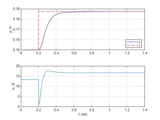
Simulate the nonlinear response with the gain-scheduled PID. The MaglevClosedLoop.slx model uses the LPV System block for the controller.

Specify initial conditions and simulate the model.

h0 = (hmin+hmax)/2;
hdot0 = 0;
tstep = 0.2;
Tf = 1.2;
hstep0 = h0;
hStepAmp = 0.25*h0;
hstepf = h0+hStepAmp;
sim('MaglevClosedLoop',[0 tstep+Tf]);

Plot the responses.

figure(3);
subplot(2,1,1);
plot(y.Time,y.Data,'b',r.Time,r.Data,'r--');
ylabel('y, m');
legend('y','r','Location','Southeast');
grid on;
subplot(2,1,2);
plot(u.Time,u.Data);
ylabel('u, A');
xlabel('t, sec');
grid on;

Figure contains 2 axes objects. Axes object 1 with ylabel y, m contains 2 objects of type line. These objects represent y, r. Axes object 2 with xlabel t, sec, ylabel u, A contains an object of type line.

Compare results with the LPV simulation.

CL = Tlpv*Fref;

Set $p (t)$ to an ideal trajectory and simulate the step response.

t = linspace(0,tstep+Tf,100);
StepConfig = RespConfig('Bias',h0,'Delay',tstep,'Amplitude',hStepAmp);
p_ideal = step(Tideal*Fref,t,StepConfig);
y1 = step(CL,t,p_ideal,StepConfig);

Set $p (t) = h (t)$ and simulate the step response.

pFcn = @(t,x,u) x(1);
StepConfig = RespConfig('Bias',h0,'Delay',tstep,...
   'Amplitude',hStepAmp,'InitialParameter',h0);
y2 = step(CL,t,pFcn,StepConfig);

Plot the response comparison.

figure(4)
tsim = y.Time;
ysim = y.Data;
plot(t,y1,t,y2,tsim,ysim,'k--');
legend('p ideal','p true','Nonlinear','Location','Southeast');
xlim([0 Tf]), grid

Figure contains an axes object. The axes object contains 3 objects of type line. These objects represent p ideal, p true, Nonlinear.

Both LPV simulations approximate the nonlinear response well. The simulation with the true trajectory provides a slightly better approximation.

Close the models.

bdclose('MaglevOpenLoop')
bdclose('MaglevClosedLoop')