根轨迹设计
根轨迹设计是一种常见的控制系统设计方法,利用该方法,您可以在根轨迹图中编辑补偿器增益、极点和零点。
当控制系统的开环增益 k 在连续值范围内变化时,根轨迹图显示反馈系统闭环极点的轨迹。例如,在以下跟踪系统中:
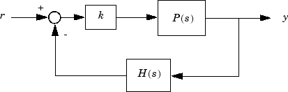
P(s) 是被控对象,H(s) 是传感器动态特性,k 是可调标量增益。闭环极点是下式的根:
根轨迹方法包括在复平面上绘制闭环极点随 k 变化的轨迹。您可以使用该图确定与期望的闭环极点集相关的增益值。
此示例说明如何使用根轨迹图形调节方法为电液伺服机构设计补偿器。
被控对象模型
简化版本的电液伺服机构模型包括以下组件:
推挽放大器(一对电磁铁)
位于高压液压油腔中的滑动阀芯
油腔中用于液压油流动的阀门开口
带有活塞驱动柱塞的中心腔室,用于向负载施加力
对称的回油腔

阀芯上的力与电磁铁线圈中的电流成正比。当阀芯运动时,阀门打开,使高压液压油流入腔室。流动的液压油推动活塞向阀芯的相反方向运动。有关此模型的详细信息,包括线性化模型的推导过程,请参阅[1]。
您可以使用电磁铁的输入电压来控制柱塞位置。当柱塞位置测量值可用时,您可以使用反馈进行柱塞位置控制,如下图所示,其中 Gservo 表示伺服机构:

设计需求
对于此示例,需要调节补偿器 C(s) 以满足以下闭环阶跃响应需求:
2% 的稳定时间小于 0.05 秒。
最大超调量小于 5%。
打开控制系统设计器
在 MATLAB® 命令行中,加载伺服机构的线性化模型,并以根轨迹编辑器配置打开控制系统设计器。
load ltiexamples Gservo
controlSystemDesigner("rlocus",Gservo);
该 App 会打开,并将 Gservo 作为默认控制架构 (Configuration 1) 的被控对象模型导入。
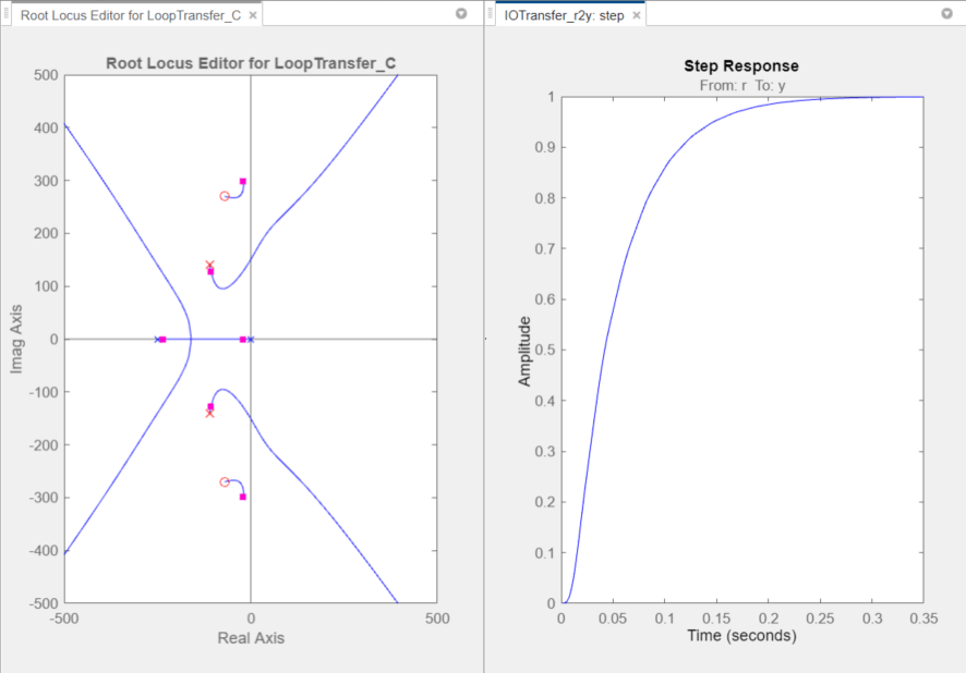
在控制系统设计器中,根轨迹编辑器图和输入-输出阶跃响应会打开。
要同时查看开环频率响应和闭环阶跃响应,请点击图并将其拖动到所需位置。
该 App 会并排显示波特编辑器和阶跃响应图。

在闭环阶跃响应图中,上升时间约为 2 秒,不满足设计需求。
为使根轨迹图更易于阅读,请放大显示。在根轨迹编辑器中,右键点击绘图区域并选择属性。
在“属性编辑器”对话框的范围选项卡中,将实轴范围和虚轴范围指定为 -500 至 500。
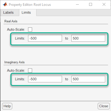
点击关闭。
增大增益
为获得更快的响应,增大补偿器增益。在根轨迹编辑器中,右键点击绘图区域并选择编辑补偿器。
在“补偿器编辑器”对话框中,将增益指定为 20。

在根轨迹编辑器图中,闭环极点位置会移动以反映新的增益值。同时,阶跃响应图会更新。

闭环响应不满足稳定时间需求,并呈现不需要的振铃。
增大增益会使系统欠阻尼,进一步增大会导致不稳定。因此,为满足设计需求,您必须指定附加的补偿器动态特性。有关添加和编辑补偿器动态特性的详细信息,请参阅Edit Compensator Dynamics in Control System Designer。
添加极点
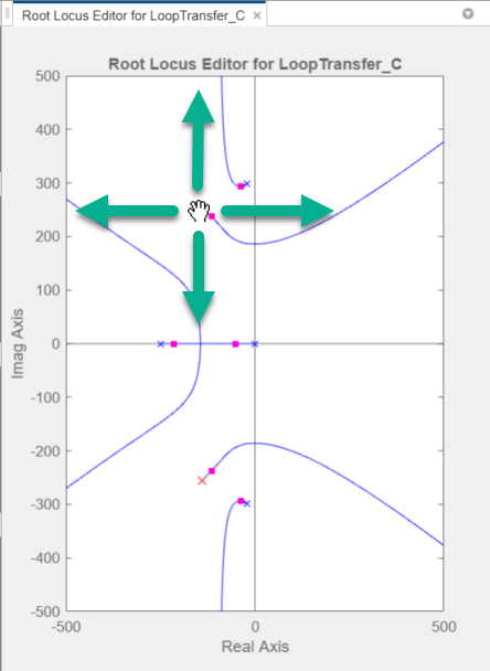
要为补偿器添加复极点对组,请在根轨迹编辑器中,右键点击绘图区域并选择添加极点或零点 > 复极点。点击要添加其中一个复极点的绘图区域位置。

该 App 会将复极点对组作为红色 X 标记添加到根轨迹图,并更新阶跃响应图。
在根轨迹编辑器中,将新极点拖动到 –140 ± 260i 附近的位置。拖动一个极点时,另一个极点会自动更新。
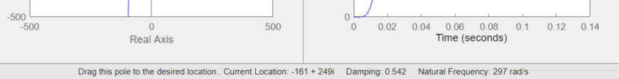
提示
当您拖动极点或零点时,该 App 会在右侧状态栏中显示新值。
添加零点
要为补偿器添加复零点对组,请在“补偿器编辑器”对话框中,右键点击动态特性表,然后选择添加极点或零点 > 复零点。

该 App 会将 –1 ± i 处的一对复零点添加到补偿器。
在动态特性表中,点击复零点行。然后在编辑所选动态特性部分中,将实部指定为 -170,将虚部指定为 430。
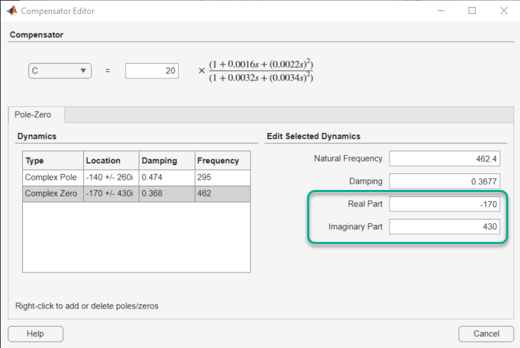
补偿器和响应图会自动更新以反映新的零点位置。

在阶跃响应图中,稳定时间约为 0.1 秒,不满足设计需求。
调整零极点
补偿器设计过程可能涉及一些试错。请调整补偿器增益、极点位置和零点位置,直到满足设计标准。
满足设计需求的一种可能的补偿器设计为:
补偿器增益为
10复极点位于 –110 ± 140i 处
复零点位于 –70 ± 270i 处
在“补偿器编辑器”对话框中,使用这些值配置您的补偿器。在阶跃响应图中,稳定时间约为 0.05 秒。
要验证确切的稳定时间,请右键点击阶跃响应图区域,然后选择特征 > 稳定时间。稳定时间指示器会出现在响应图上。
要查看稳定时间,请将光标悬停在稳定时间指示器上。
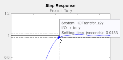
稳定时间约为 0.043 秒,满足设计需求。
参考
[1] Clark, R. N. Control System Dynamics, Cambridge University Press, 1996.