Fit Logarithmic Models
About Logarithmic Models
A logarithmic model has a steep initial period of growth before continuing to grow at a slower rate. Logarithmic models are used in a variety of applications, such as studies of population growth and signal processing. Curve Fitting Toolbox™ supports the logarithmic models described in the following table.
| Logarithmic Model | Base | Equation |
|---|---|---|
Natural Log | e | Y = a*log(x)+b |
| Common Log | 10 | Y = a*log10(x)+b |
| Binary Log | 2 | Y = a*log2(x)+b |
In the above equations, a is a scaling
parameter and b is the value for Y
when x = 1. You can convert between the different
logarithmic models using the change of base formula , where j is the base of the model to
convert to, and i is the base of the model being
converted. The logarithmic model you use to fit to your data depends on the
type of problem you are solving.
Fit Logarithmic Models Using Curve Fitter
Generate some noisy data by using the linspace, log2, and randn functions.
rng(0,"twister") %  For reproducibility
x = linspace(0.01,3,100)';
y = log2(x) + 0.2*randn(100,1);
Open the Curve Fitter app from the command line.
curveFitter
Alternatively, on the Apps tab, in the Math, Statistics and Optimization group, click Curve Fitter.
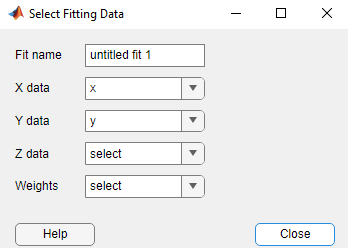
In the Curve Fitter app, select the data variables for the fit. On the Curve Fitter tab, in the Data section, click Select Data. In the Select Fitting Data dialog box, select x as the X data value and y as the Y data value.

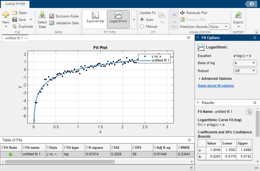
The app plots the data points as you select variables. By default, the app fits a polynomial to the data. To fit a logarithmic model, click Logarithmic in the Fit Type section of the Curve Fitter tab.

The app fits a natural log model.

The fitted natural log model increases relatively quickly for small values of x. The Results panel shows the formula for the natural log model and the fitted coefficients with 95% intervals. The Table of Fits shows that the fitted model has a sum of squares error (SSE) of approximately 5.2, and an R-square value of approximately 0.97.
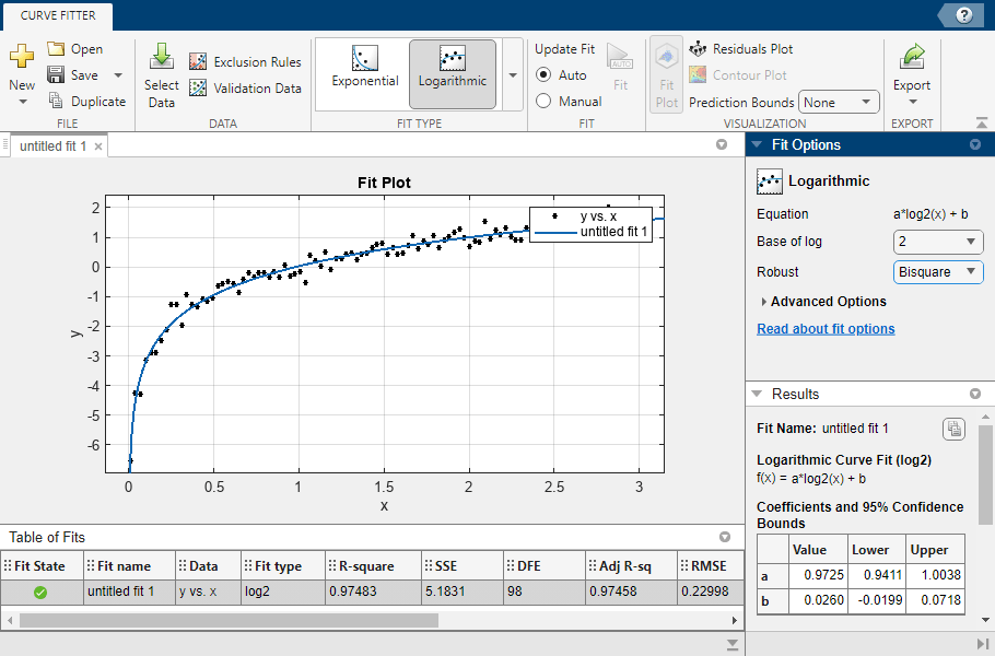
To compare the natural log model with a binary log model, select 2 for Base of log in the Fit Options panel. The app fits a binary log model to the data.

The Table of Fits shows that the fitted natural log model and the fitted binary log model have the same SSE and R-square values. The plot also indicates that the fitted models are the same. The only differences between the models are the base of the logarithmic model and the values and confidence bounds for the coefficient a. You can manually convert between the natural log model and the binary log model by using the equations and .
By default, the app uses linear least-squares fitting to calculate the fitted coefficients. You can select a robust fitting method from the Robust menu in the Fit Options panel. For example, to use the bisquare-weights method, select Bisquare.

The Table of Fits shows that the SSE for the binary log model is slightly smaller with bisquare-weights fitting than with linear least-squares fitting, and that the R-square value is slightly larger.
Fit Logarithmic Models from Command Line
Generate some noisy data by using the linspace, log10, and randn functions.
rng(0,"twister") %  For reproducibility
x = linspace(0.01,3,100)';
y = log10(x) + 0.1*randn(100,1);
Fit a common log model to the data.
f = fit(x,y,"log10")f =
Linear model Log10:
f(x) = a*log10(x) + b
Coefficients (with 95% confidence bounds):
a = 0.9561 (0.9039, 1.008)
b = 0.01415 (-0.008812, 0.03712)
f is a cfit object that contains the results of fitting the common log model to the data. The output displays the formula for the common log model and the fitted coefficients with 95% confidence bounds.
Plot f and the data.
plot(f,x,y)

The plot shows that f follows the bulk of the data.
See Also
Apps
Functions
fit|fittype|fitoptions