Compare Solvers for Classifying Images Using Experiment
This example shows how to train a deep learning network for classification by using Experiment Manager. In this example, you train two networks to classify images of MathWorks merchandise into five classes. Each network is trained using three algorithms. In each case, a confusion matrix compares the true classes for a set of validation images with the classes predicted by the trained network.
This experiment requires the Deep Learning Toolbox™ Model for GoogLeNet Network support package. Before you run the experiment, install this support package by calling the googlenet function and clicking the download link.
Create Built-in Training Experiment
You can quickly configure an image classification experiment by using a template on the Experiment Manager start page. Open the Experiment Manager app. Then, click New > Blank Project, and choose the Image Classification by Sweeping Hyperparameters template. This experiment is a built-in training experiment, so it uses the trainnet function to train a neural network for each experiment trial. This template automatically generates an experiment that includes a sample initialization function, a default hyperparameter, and a setup function designed for image classification.
Author Experiment Description
In the Description section of the experiment editor, write a textual description of the experiment.
Merchandise image classification using:
* an untrained network (default) or a pretrained network (googlenet)
* various solvers for training networks (sgdm, rmsprop, or adam)
Configure Initialization Function
The Initialization Function section of the experiment editor specifies a function that contains setup code to execute before the experiment trials begin.
In the initialization function:
Load and unzip a data set that contains 75 images of MathWorks merchandise belonging to five different classes.
Define image datastores containing training and validation data.
Return the experiment data as a scalar structure
output, which you can access in the setup function.
function output = Experiment1Initialization1
filename = "MerchData.zip";
dataFolder = fullfile(tempdir,'MerchData');
unzip(filename,tempdir);

imds = imageDatastore(dataFolder, ...
    IncludeSubfolders=true, ....
    LabelSource="foldernames");

numTrainingFiles = 0.7;
[output.imdsTrain,output.imdsValidation] = splitEachLabel(imds,numTrainingFiles);
end
Specify Hyperparameters
The Hyperparameters section specifies the strategy and hyperparameter values to use for the experiment. When you run the experiment, Experiment Manager trains the network using every combination of hyperparameter values specified in the hyperparameter table.
For this example, click Add twice, and configure the network and solver hyperparameters.
Name | Values |
|---|---|
|
|
|
|
Configure Setup Function
The Setup Function section specifies a function that configures the training data, network architecture, loss, and training options for the experiment. To open this function in the Editor, click Edit.
In the setup function:
Specify the input as the structure
params, which has three fields. TheInitializationFunctionOutputfield is the scalar structure returned by the initialization function. Thenetworkandsolverfields are hyperparameters defined in the table in the Hyperparameter section.Return four outputs that the
trainnetfunction uses to train a network.Load the sample data that was returned by the initialization function and passed to the setup function as a field of the input argument
params.Define the convolutional neural network architecture specified by the hyperparameter
network.For classification tasks, use cross-entropy loss.
Train the network by using the algorithm specified by the hyperparameter
Solver.
function [imdsTrain,layers,lossFcn,options] = Experiment1_setup1(params)
data = params.InitializationFunctionOutput;
imdsTrain = data.imdsTrain;
imdsValidation = data.imdsValidation;
numClasses = 5;

switch params.network
    case "default"
        inputSize = [227 227 3];
        layers = [
            imageInputLayer(inputSize)
            convolution2dLayer(5,20)
            batchNormalizationLayer
            reluLayer
            fullyConnectedLayer(numClasses)
            softmaxLayer];
    case "googlenet"
        layers = imagePretrainedNetwork("googlenet",NumClasses=numClasses);
    otherwise
        error("Undefined network selection.");
end

lossFcn = "crossentropy";

options = trainingOptions(params.solver, ...
    MiniBatchSize=10, ...
    MaxEpochs=8, ...
    InitialLearnRate=1e-4, ...
    Shuffle="every-epoch", ...
    ValidationData=imdsValidation, ...
    ValidationFrequency=5, ...
    Verbose=false);
end
Run Experiment
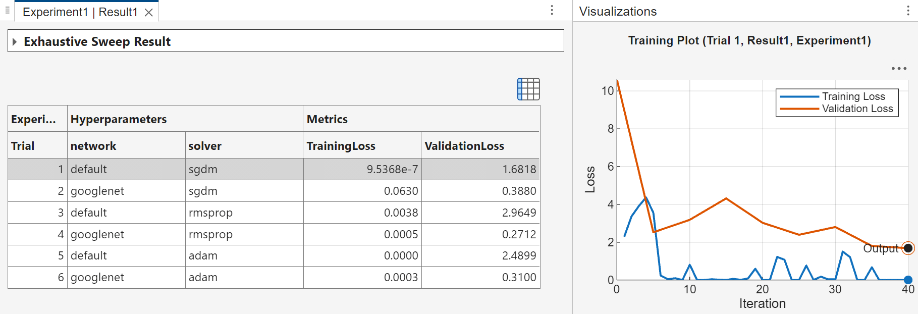
When you run the experiment, Experiment Manager trains the network defined by the setup function six times. Each trial uses a different combination of hyperparameter values. A table of results displays the accuracy and loss for each trial.
To visualize the progress of a trial while the experiment is running, select a trial in the table of results. Then, on the Review Results section of the toolstrip, click Training Plot. You can show or hide columns by clicking the ![]() button above the table.
button above the table.
By default, Experiment Manager runs one trial at a time. For information about running multiple trials at the same time or offloading your experiment as a batch job in a cluster, see Run Experiments in Parallel and Offload Experiments as Batch Jobs to a Cluster.
Evaluate Results
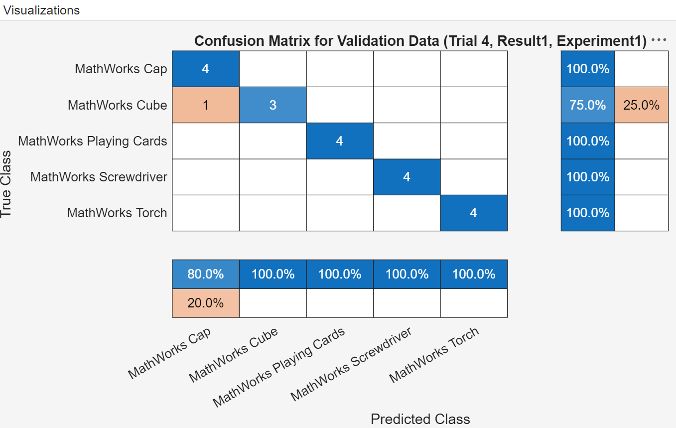
This experiment creates a confusion matrix for each trial which you can use to evaluate the quality of the network. Select a trial, and on the Review Results section of the toolstrip, click Validation Data.
To find the best result for your experiment, sort the table of results by validation accuracy. In the table of results, point to the header of the Validation Accuracy variable, click the sort icon, and select the Sort in Descending Order. The trial with the highest validation accuracy appears at the top of the results table.