Convert Convolutional Network to Spiking Neural Network

Since R2023b

This example shows how to convert a conventional convolutional neural network (CNN) to a spiking neural network (SNN).

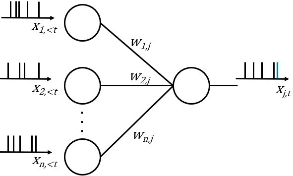
SNNs are neural networks that closely mimic biological neural networks. In SNNs, information is encoded in the timing of spikes and data is passed through the networks in the form of sparse sequences known as Poisson spike trains. Spikes received at a neuron contribute to the membrane potential of the neuron and the neuron emits a spike or fires when the membrane potential reaches a threshold values. This figure shows a dynamic neuron spiking process.

Schematic diagram of a dynamic neuron spiking process.

Deploying SNNs on specialized hardware, called neuromorphic hardware, has many advantages, such as low power consumption and fast inference. Applications of SNNs include processing event-driven information, such as input from neuromorphic vision sensors for optical flow estimation, tracking, and gesture recognition [1]. You can also use SNNs as a low-power alternative to typical artificial neural networks in cases where power efficiency is a favorable property, such as in battery-powered robotics and battery-powered embedded hardware.

Training algorithms for SNNs include these options:

Direct supervised learning algorithms. These algorithms perform supervised learning on the SNN, typically using variations of conventional backpropagation algorithms [2].
Unsupervised learning algorithms. These algorithms typically involve spike-time-dependent plasticity (STDP) [3].
Rate-based learning algorithms. These algorithms typically involve training a typical ANN using backpropagation and then converting it to an SNN, which you use only for inference [4].

In this example, you use a rate-based learning algorithm to train a conventional convolutional neural network (CNN) to classify images. You then replace and add layers to convert the network to an SNN and then classify images using the SNN. The conversion techniques you use are based on those outlined in [4].

Load Training and Testing Data

Load the training and testing data sets. Each data set contains 5000 28-by-28 pixel grayscale images of handwritten digits 0-9. The data sets also contain associated labels denoting which digit the image represents (0-9). These data sets are attached to the example as supporting files. Open the example as a live script to access the supporting files.

load("DigitsDataTrain")
load("DigitsDataTest")

Store the class labels.

classes = string(unique(labelsTrain));

Display some of the images in the training data set.

perm = randperm(5000,12);
figure;
tiledlayout("flow")
for idx = 1:12
    nexttile
    imshow(XTrain(:,:,:,perm(idx)));
end

Examine Integrate-and-Fire Model

The network architecture is informed by the spiking neuron model. The spiking neuron model in this example is the simple integrate-and-fire (IF) model [4]. This equation defines the evolution of the membrane voltage:

$\frac{d}{d t} v_{mem} (t) = \sum_{i} \sum_{s \in S_{i}} w_{i} δ (t - s),$

where $w_{i}$ is the weight of the $i$ th incoming synapse, $δ (\cdot)$ is the delta function, and $S_{i} = {t_{i}^{0}, t_{i}^{1}, . . .}$ contains the spike times of the $i$ th presynaptic neuron. If the membrane voltage crosses the spiking threshold $v_{thr}$ , a spike is generated and the membrane voltage is reset to a reset potential $v_{res}$ . In this example, you discretize the continuous-time description of the IF model into simulation steps.

Define Network Architecture

To reduce the accuracy lost when you convert the network to an SNN, the network architecture meets these constraints [5]:

The only activation functions are ReLU. Values that pass through a generic network can be negative, for example, the output of a convolution layer or the output of a sigmoid layer. SNNs that use an IF model cannot represent negative values. Using ReLU activation functions after convolution layers ensures that layer outputs are nonnegative.
Convolution and fully connected layers must have a fixed bias of 0, which the network does not learn during training. As with negative values, SNNs that use an IF model cannot represent bias terms.

Define the CNN architecture. Fix the bias by setting the BiasLearnRateFactor property of each convolution layer to 0.

inputSize = size(XTrain,1,2,3);

layers = [imageInputLayer(inputSize,Normalization="none")
    convolution2dLayer([5 5],12,BiasLearnRateFactor=0)
    reluLayer
    averagePooling2dLayer([2 2])
    convolution2dLayer([5 5],64,BiasLearnRateFactor=0)
    reluLayer
    averagePooling2dLayer([2 2])
    fullyConnectedLayer(10,BiasLearnRateFactor=0)
    softmaxLayer];

Specify Training Options

Specify the training options to match those in [4], with the exception of the learning rate, which is set to 0.05 instead of 1.

trainingOpts = trainingOptions("sgdm", ...
    MaxEpochs=15, ...
    InitialLearnRate=0.05, ...
    Momentum=0.5, ...
    MiniBatchSize=40, ...
    Plots="training-progress", ...
    Verbose=false);

Train Network

Train the network.

net = trainnet(XTrain,labelsTrain,layers,"crossentropy",trainingOpts);

Test Network

Evaluate the network performance on the test data set and compare the predicted labels to the true labels.

YPred = predict(net,XTest);
labelsPred = onehotdecode(YPred,classes,2);
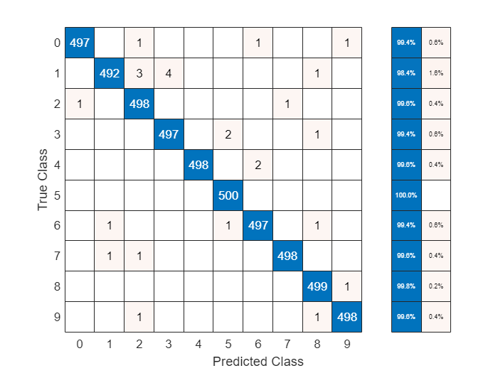
cnnAccuracy = sum(labelsPred == labelsTest)/numel(labelsTest)

cnnAccuracy = 0.9948

Visualize the results in a confusion chart.

figure
confusionchart(labelsTest,labelsPred,RowSummary="row-normalized")

Convert Network to SNN

To convert the CNN to an SNN, perform these steps:

Add an intermediate layer that converts image to Poisson spike trains after the first layer. The intermediate layer is a SpikeConversionLayer object. The object definition is attached to this example as a supporting file. The spikeThreshold variable controls the sparsity of the generated spike trains.
Convert all the layers in the network to spiking layers, ignoring the activation layers and the output layers. To convert the layers, wrap each original layer in a SpikingLayer object, which overloads the predict method of the underlying layer object to apply spiking behavior. The object definition is attached to this example as a supporting file. To learn how the spikes are transmitted, open the SpikingLayer MAT-file and inspect the predict method.

spikeThreshold = 2.5;

layers = [
    net.Layers(1)
    SpikeConversionLayer(spikeThreshold);
    SpikingLayer(net.Layers(2))
    SpikingLayer(net.Layers(4))
    SpikingLayer(net.Layers(5))
    SpikingLayer(net.Layers(7))
    SpikingLayer(net.Layers(8))];

snn = dlnetwork(layers);

Select a random image from the test data set.

imageIdx = ceil(size(XTest,4)*rand);

Generate three sets of spikes using the SpikeConversionLayer from the selected image and visualize the results.

figure
tiledlayout("flow")

nexttile
imshow(XTest(:,:,:,imageIdx))
title("Original Image")

for idx = 1:3

    exampleSpikeTrain = predict(snn,XTest(:,:,:,imageIdx),Outputs=snn.Layers(2).Name);

    nexttile
    imshow(exampleSpikeTrain)
    title("Generated Spikes")

end

Classify Test Image Using SNN

SNNs predict using a simulation. During the simulation, the software passes an image to be classified through the network multiple times, until the network starts spiking at the output. The node on the output layer that spikes more than the other nodes determines the classification.

Define the parameters of the simulation. In [4], the simulation options are defined in terms of time, with a total simulation duration of 0.04 ms and a simulation time step of 0.001 ms. To simplify the subsequent code, define the total number of simulation steps only.

totalSteps = 40;

Predict the class of the image. For each simulation step, pass the image through the network using the predict function and update the state of the network.

for simulationStep = 1:totalSteps
    [~,state] = predict(snn,XTest(:,:,:,imageIdx));
    snn.State = state;
end

Get the prediction by finding the output neuron that records the most spikes.

[~,idx] = max(snn.Layers(end).SumSpikes,[],1);
labelsPred = categorical(idx,1:10,categories(labelsTest))

labelsPred = categorical
     2

Classify Multiple Test Images Using SNN

To classify all the images in the test data set, pass all of the images through the network.

The network still contains spikes from the previous classification. To clear the spikes, recreate the SNN.

snn = dlnetwork(layers);

Initialize simulations metrics.

snnAccuracy - SNN accuracy at each simulation step, specified as a vector.
snnConfusionMat - Confusion chart of the network at each simulation step, specified as a matrix.

numClasses = length(categories(labelsPred));
snnAccuracy = zeros(1,totalSteps);
snnConfusionMat = zeros(numClasses,numClasses,totalSteps);

Initialize a plot of the network accuracy and a confusion chart.

accuracyFigure = figure;
ax = axes(accuracyFigure);
lineAccuracySimulation = animatedline(ax);
ylim([0 1])
xlabel("Simulation Time Step")
ylabel("Accuracy")
grid on

confusionChart = figure;

Pass all of the test images through the network totalSteps times. After each simulation step, update the accuracy plot and the confusion chart.

for simulationStep = 1:totalSteps

    % Pass input images through the network.
    [~,state] = predict(snn,XTest);
    snn.State = state;

    % Get prediction by using the output node with the most spikes.
    [~,idx] = max(snn.Layers(end).SumSpikes,[],1);
    labelsPred = categorical(idx,1:10,categories(labelsTest));

    % Calculate and display the network accuracy.
    snnAccuracy(simulationStep) = sum(labelsPred == labelsTest')/numel(labelsTest);
    addpoints(lineAccuracySimulation,simulationStep,snnAccuracy(simulationStep))
    title(ax,"SNN Accuracy After " + simulationStep + " Simulation Steps: " + snnAccuracy(simulationStep))

  
    % Calculate and display the confusion chart.
    [snnConfusionMat(:,:,simulationStep),order] = confusionmat(labelsTest,labelsPred');
    cm = confusionchart(confusionChart,snnConfusionMat(:,:,simulationStep),categories(labelsPred),RowSummary="row-normalized");
    title(cm,"SNN Confusion Chart After " + simulationStep + " Simulation Steps")
    drawnow

end

References

[1] Pfeiffer, Michael, and Thomas Pfeil. “Deep Learning With Spiking Neurons: Opportunities and Challenges.” Frontiers in Neuroscience 12 (October 25, 2018): 774. https://doi.org/10.3389/fnins.2018.00774.

[2] Lee, Jun Haeng, Tobi Delbruck, and Michael Pfeiffer. “Training Deep Spiking Neural Networks Using Backpropagation.” Frontiers in Neuroscience 10 (November 8, 2016). https://doi.org/10.3389/fnins.2016.00508.

[3] Diehl, Peter U., and Matthew Cook. “Unsupervised Learning of Digit Recognition Using Spike-Timing-Dependent Plasticity.” Frontiers in Computational Neuroscience 9 (August 3, 2015). https://doi.org/10.3389/fncom.2015.00099.

[4] Diehl, Peter U., Daniel Neil, Jonathan Binas, Matthew Cook, Shih-Chii Liu, and Michael Pfeiffer. “Fast-Classifying, High-Accuracy Spiking Deep Networks through Weight and Threshold Balancing.” In 2015 International Joint Conference on Neural Networks (IJCNN), 1-8. Killarney, Ireland: IEEE, 2015. https://doi.org/10.1109/IJCNN.2015.7280696.

[5] Cao, Yongqiang, Yang Chen, and Deepak Khosla. “Spiking Deep Convolutional Neural Networks for Energy-Efficient Object Recognition.” International Journal of Computer Vision 113, no. 1 (May 2015): 54-66. https://doi.org/10.1007/s11263-014-0788-3.