Train Bayesian Neural Network
This example shows how to train a Bayesian neural network (BNN) for image regression using Bayes by backpropagation [1]. You can use a BNN to predict the rotation of handwritten digits and model the uncertainty of those predictions.
A Bayesian neural network (BNN) is a type of deep learning network that uses Bayesian methods to quantify the uncertainty in the predictions of a deep learning network. This example uses Bayes by backpropagation (also known as Bayes by backprop) to estimate the distribution of the weights of a neural network. By using a distribution of weights instead of a single set of weights, you can estimate the uncertainty of the network predictions.
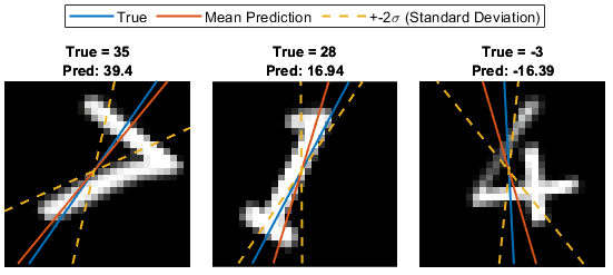
This figure shows an example of the predicted angles of rotation and the uncertainty regions for an estimated distribution of weights.

Load Data
Load the digits data set. This data set contains synthetic images of handwritten digits together with the corresponding angles (in degrees) by which each image is rotated.
Load the training and test images as 4-D arrays. The variables anglesTrain and anglesTest outputs are the rotation angles in degrees. The training and test data sets each contain 5000 images.
load DigitsDataTrain
load DigitsDataTest
Create a single datastore that contains the training predictors and responses. To convert numeric arrays to datastores, use arrayDatastore. Then, use the combine function to combine these datastores into a single datastore.
dsXTrain = arrayDatastore(XTrain,IterationDimension=4);
dsTTrain = arrayDatastore(anglesTrain);
dsTrain = combine(dsXTrain,dsTTrain);
Extract the size of the responses and the number of observations.
numResponses = size(anglesTrain,2)
numResponses =
1
numObservations = numel(anglesTrain)
numObservations =
5000
Display 64 random training images.
idx = randperm(numObservations,64);
I = imtile(XTrain(:,:,:,idx));
figure
imshow(I)

Define Network Architecture
To model the weights and biases using a distribution rather than a single deterministic set, you must define a probability distribution for the weights. You can define the distribution using Bayes' theorem:
where is the likelihood and is the prior distribution. In this example, you set the weights and biases to follow a Gaussian distribution (corresponding to squared-loss). During training, the network learns the means and variances of the Gaussian distributions, which determine the distributions of the weights and biases.
Set the prior to a Gaussian mixture model [1] with two components, each with a mean of 0 and variances sigma1 and sigma2. You can fix the variances before training or learn them during training. Both components of the mixture model have a mixing proportion of 0.5.
Define a Bayesian neural network for image regression.
For image input, specify an image input layer with an input size matching the training data.
Do not normalize the image input. Set the
Normalizationoption of the input layer to"none".Specify three Bayes fully connected layers with ReLU activation layers between them.
A Bayes fully connected layer is a type of fully connected layer that stores the average weights and biases of the expected distribution of the weights. When computing the activations of the layer, the software shifts the mean weights and biases by random Gaussian noise and uses the shifted weights and biases to compute the outputs of the layer.
To create a Bayes fully connected layer, use the bayesFullyConnectedLayer.m custom layer, attached to this example as a supporting file. The Bayes fully connected layer takes as input the output size and the parameters of the prior probabilities of the weight distribution, sigma1 and sigma2.
Define the network.
inputSize = [28 28 1];
outputSize = 784;

sigma1 = 1;
sigma2 = 0.5;

layers = [
    imageInputLayer(inputSize,Normalization="none")
    bayesFullyConnectedLayer(outputSize,Sigma1=sigma1,Sigma2=sigma2)
    reluLayer
    bayesFullyConnectedLayer(outputSize/2,Sigma1=sigma1,Sigma2=sigma2)
    reluLayer
    bayesFullyConnectedLayer(1,Sigma1=sigma1,Sigma2=sigma2)];
Create a dlnetwork object from the layer array.
net = dlnetwork(layers);
Visualize the network using analyzeNetwork. You can see that the learnables for the Bayes fully connected layers include the means and variances for the weights and biases.
analyzeNetwork(net)

Define Learnable Parameters
The learnable parameters comprise network (layer) learnables and global learnables. During training, the algorithm updates these learnable parameters:
The means and variances of the layer weights and biases (per layer)
The prior probabilities for the weight distributions (per layer)
The sampling noise (global)
Initialize Sampling Noise
Use sampling noise to represent the noise in the predictions of the neural network. Learn the sampling noise with the network weights and biases.
Initialize the sampling noise.
samplingNoise = dlarray(1);
Initialize Prior Probability
You can fix the prior variance parameters or learn them during training like the other learnable parameters. Learn the prior parameters during training using a small learn rate so that their values remain close to the initial values. Set the initial learn rate to 0.25.
doLearnPrior = true;
priorLearnRate = 0.25;

numLearnables = size(net.Learnables,1);

for i=1:numLearnables
    layerName = net.Learnables.Layer(i);
    parameterName = net.Learnables.Parameter(i);

    if parameterName == "Sigma1" || parameterName == "Sigma2"
        if doLearnPrior
            net = setLearnRateFactor(net,layerName,parameterName,priorLearnRate);
        else
            net = setLearnRateFactor(net,layerName,parameterName,0);
        end
    end
end
Define Model Loss Functions
Define a function that returns the model loss and the gradients of the loss with respect to the learnable parameters. In this example, you minimize the evidence lower bound (ELBO) loss defined in the Evidence Lower Bound Loss section.
Create the function modelLoss, listed in the Model Loss Function section. The function takes as input a dlnetwork object and a mini-batch of input data with corresponding targets. The function returns these values:
ELBO loss
Root mean squared error (RMSE)
Gradients of the loss with respect to the learnable parameters
Gradients of the loss with respect to the sampling noise
Network state
Specify Training Options
Train for 50 epochs with a mini-batch size of 128.
numEpochs = 50;
miniBatchSize = 128;
Track the ELBO loss during training. Plot the loss every 50 iterations and average the loss across five samples of the learnable parameters.
numSamplesForavgELBO = 5;
averageLossComputationFrequency = 50;
Train Model
Create a minibatchqueue object to process and manage the mini-batches of images. For each mini-batch:
Use the custom mini-batch preprocessing function
preprocessMiniBatch(defined at the end of this example) to one-hot encode the class labels.Format the image data with the dimension labels
"SSCB"(spatial, spatial, channel, batch). By default, theminibatchqueueobject converts the data todlarrayobjects with underlying type single.Train on a GPU if one is available. By default, the
minibatchqueueobject converts each output to agpuArrayobject if a GPU is available. Using a GPU requires a Parallel Computing Toolbox™ license and a supported GPU device. For information on supported devices, see GPU Computing Requirements (Parallel Computing Toolbox).
mbq = minibatchqueue(dsTrain, ...
    MiniBatchSize=miniBatchSize, ...
    MiniBatchFcn=@preprocessMiniBatch, ...
    MiniBatchFormat=["SSCB" "CB"]);
Initialize the parameters for Adam optimization.
trailingAvg = [];
trailingAvgSq = [];
trailingAvgNoise = [];
trailingAvgNoiseSq = [];
Calculate the total number of iterations for the training progress monitor.
numIterationsPerEpoch = ceil(numObservations/miniBatchSize);
numIterations = numEpochs*numIterationsPerEpoch;
Initialize the training progress monitor.
monitor = trainingProgressMonitor( ...
    Metrics=["RMSE","AverageELBOLoss"], ...
    Info="Epoch", ...
    XLabel="Iteration");
Train the model using a custom training loop. For each epoch, shuffle the data and loop over mini-batches of data. At the end of each iteration, display the training progress. For each mini-batch:
Evaluate the model loss and gradients using
dlfevaland themodelLossfunction.Update the network parameters using the
adamupdatefunction.Update the sampling noise parameters (global parameters) using the
adamupdatefunction.Record the RMSE and the average ELBO loss.
iteration = 0;
epoch = 0;

% Loop over epochs.
while epoch < numEpochs && ~monitor.Stop
    epoch = epoch + 1;
    miniBatchIdx = 0;

    % Shuffle data.
    shuffle(mbq);

    while hasdata(mbq) && ~monitor.Stop
        iteration = iteration + 1;
        miniBatchIdx = miniBatchIdx + 1;

        [X,T] = next(mbq);

        [elboLoss,rmsError,gradientsNet,gradientsNoise] = dlfeval(@modelLoss, ...
            net,X,T,samplingNoise,miniBatchIdx,numIterationsPerEpoch);

        % Update the network parameters using the Adam optimizer.
        [net,trailingAvg,trailingAvgSq] = adamupdate(net,gradientsNet, ...
            trailingAvg,trailingAvgSq,iteration);

        % Update the sampling noise.
        [samplingNoise,trailingAvgNoise,trailingAvgNoiseSq] = adamupdate(samplingNoise, ...
            gradientsNoise,trailingAvgNoise,trailingAvgNoiseSq,iteration);

        % Record the RMSE.
        recordMetrics(monitor,iteration,RMSE=double(rmsError))

        % Record the average ELBO loss.
        if mod(iteration,averageLossComputationFrequency) == 0
            avgELBOLoss = averageNegativeELBO(net,X,T,samplingNoise,miniBatchIdx, ...
                numIterationsPerEpoch,numSamplesForavgELBO);

            recordMetrics(monitor,iteration,AverageELBOLoss=double(avgELBOLoss))
        end

        % Update the epoch and progress values in the monitor.
        updateInfo(monitor,Epoch=string(epoch) + " of " + string(numEpochs))
        monitor.Progress = 100*(iteration/numIterations);
    end
end

Test Network
BNNs learn the probability distribution of the weights rather than optimizing a single set of weights like convolutional neural networks. Therefore, you can view a BNN as an ensemble of networks where you sample each network from the learned probability distribution of the learnable parameters.
To test the accuracy of a BNN, generate samples for the weights and biases and compare the average prediction across the samples with the true value. The standard deviation across the predictions is the model uncertainty. Use the modelPosteriorSample function listed in the Model Prediction Function section to generate predictions for a set of inputs. The function samples times from the posterior distribution of the weights and biases. For each of the samples, the function generates predictions for the input images. The predictions from a BNN use a sample of the weights and biases; therefore, the predictions include some variational noise.
Convert the test data to a dlarray object.
XTest = dlarray(XTest,"SSCB");
if canUseGPU
    XTest = gpuArray(XTest);
end
Test Single Image
Generate 10 samples for the first test image using modelPosteriorSample. The function returns 10 predictions for the angle of rotation. The final model prediction is the average value across the 10 predictions.
idx = 1;
numSamples = 10;
img = XTest(:,:,:,idx);

predictions = modelPosteriorSample(net,img,samplingNoise,numSamples);
YTestImg = mean(predictions,1);
Plot the true angle, the predicted angles, and the mean of the predictions.
figure
lineWidth = 1.5;
uncertaintyColor = "#EDB120";

I = extractdata(img);
imshow(I)
hold on

inputSize = size(img,1);
offset = inputSize/2;

thetaActual = anglesTest(idx);
plot(offset*[1 - tand(thetaActual),1 + tand(thetaActual)],[inputSize 0], ...
    LineWidth=lineWidth)

thetaPredAvg = YTestImg;
plot(offset*[1 - tand(thetaPredAvg),1 + tand(thetaPredAvg)],[inputSize 0], ...
    LineWidth=lineWidth)

for i=1:numSamples
    thetaPred = predictions(i);
    plot(offset*[1 - tand(thetaPred),1 + tand(thetaPred)],[inputSize 0],"--", ...
        Color=uncertaintyColor)
end

hold off
title("Pred: " + round(thetaPredAvg,2)+" (Mean)" + ", True: " + round(thetaActual,2))
legend(["True","Mean Prediction","Prediction"],Location="southeast")

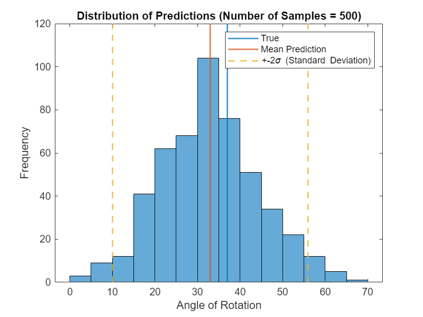
Increase the number of samples to 500 and plot the distribution of the predicted angles of rotation for the test image.
numSamples = 500;

predictions = modelPosteriorSample(net,img,samplingNoise,numSamples);
YTestImg = mean(predictions,1);
uncertaintyImg = std(predictions,1);

figure
histogram(predictions)

trueColor = "#0072BD";
predColor = "#D95319";

hold on
xline(anglesTest(idx),Color=trueColor,LineWidth=lineWidth)
xline(YTestImg,Color=predColor,LineWidth=lineWidth)
xline(YTestImg - 2*uncertaintyImg,"--",Color=uncertaintyColor,LineWidth=lineWidth)
xline(YTestImg + 2*uncertaintyImg,"--",Color=uncertaintyColor,LineWidth=lineWidth)
hold off

xlabel("Angle of Rotation")
ylabel("Frequency")
title("Distribution of Predictions (Number of Samples = " + numSamples + ")")
legend("","True","Mean Prediction","+-" + "2\sigma (Standard Deviation)")

Test All Images
Predict the angle of rotation for each test image using 100 samples of the learnable parameters.
numSamples = 100;
predictions = modelPosteriorSample(net,XTest,samplingNoise,numSamples);
YTest = mean(predictions,1);
uncertainty = std(predictions,1);
Calculate the prediction error between the true and predicted angles of rotation.
predictionError = anglesTest - YTest';
Use the RMSE to measure the differences between the true and predicted angles of rotation.
squares = predictionError.^2;
rmse = sqrt(mean(squares))
rmse =
14.9553
Visualize Predicted Angles and Uncertainties
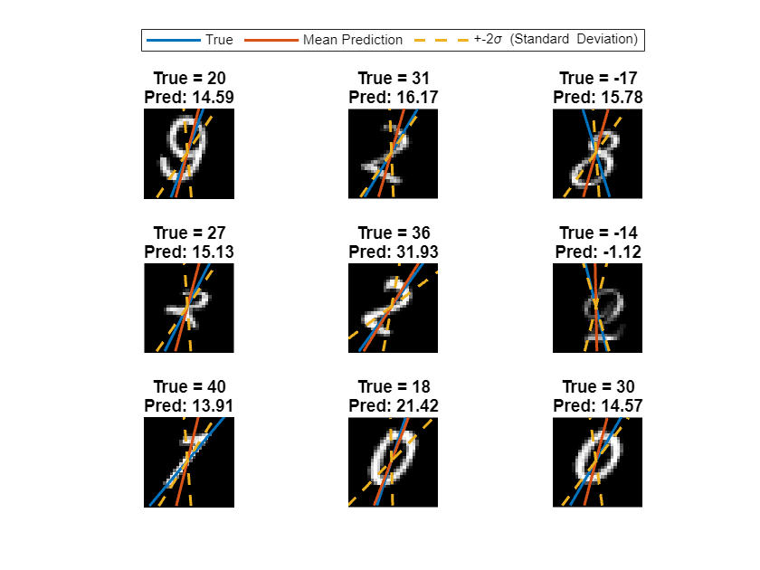
View some of the images with their predicted and true angles. Show the uncertainty in the predictions using the standard deviation of the model predictions.
numTestImages = numel(anglesTest);
numObservationToShow = 6;
idxTestSubset = randperm(numTestImages,numObservationToShow);

sdToPlot = 2;

tiledlayout("flow",TileSpacing="tight");

for i = 1:numObservationToShow
    idx = idxTestSubset(i);

    nexttile
    I = extractdata(XTest(:,:,:,idx));
    imshow(I)
    hold on

    thetaActual = anglesTest(idx);
    plot(offset*[1 - tand(thetaActual),1 + tand(thetaActual)],[inputSize 0],LineWidth=lineWidth)

    thetaPred = YTest(idx);
    plot(offset*[1 - tand(thetaPred),1 + tand(thetaPred)],[inputSize 0],LineWidth=lineWidth)

    thetaUncertainty = [thetaPred - sdToPlot*uncertainty(idx),thetaPred + sdToPlot*uncertainty(idx)];

    % Plot upper and lower bounds.
    lowerBound = [1 - tand(thetaUncertainty(1)),1 + tand(thetaUncertainty(1))];
    upperBound = [1 - tand(thetaUncertainty(2)),1 + tand(thetaUncertainty(2))];
    plot(offset*lowerBound,[inputSize 0],"--",Color=uncertaintyColor,LineWidth=lineWidth)
    plot(offset*upperBound,[inputSize 0],"--",Color=uncertaintyColor,LineWidth=lineWidth)

    hold off
    title({"True = " + round(thetaActual,2),"Pred: " + round(thetaPred,2)})
    if i == 2
        legend(["True","Mean Prediction","+-" + sdToPlot + "\sigma (Standard Deviation)"], ...
            Location="northoutside", ...
            NumColumns=3)
    end
end

Supporting Functions
Mini-Batch Preprocessing Function
The preprocessMiniBatch function preprocesses the data using these steps:
Extract the image data from the input cell array
dataXand concatenate it into a numeric array. Concatenating the image data over the fourth dimension adds a third dimension to each image, for the network to use as a singleton channel dimension.Extract angle data from the input cell arrays
dataAngand concatenate it along the second dimension into a numeric array.
function [X,A] = preprocessMiniBatch(dataX,dataAng)

X = cat(4,dataX{:});
A = cat(2,dataAng{:});

end
Model Prediction Function
The modelPosteriorSample function takes as input the dlnetwork object net, an input image X, the sampling noise samplingNoise, and the number of samples to generate numSamples. The function returns numSample predictions for the input image.
function predictions = modelPosteriorSample(net,X,samplingNoise,numSamples)

predictions = zeros(numSamples,size(X,4));

for i=1:numSamples
    Y = predict(net,X,Acceleration="none");
    sigmaY = exp(samplingNoise);
    predictions(i,:) = Y + sigmaY.*randn(size(Y));
end

end
Maximum Likelihood Estimation Function
The logLikelihood function estimates the likelihood of the network prediction given the true values and the sampling noise. The function takes as input the predictions Y, true values T, and sampling noise samplingNoise and returns the log-likelihood l.
function l = logLikelihood(Y,T,samplingNoise)

sigmaY = exp(samplingNoise);
l = sum(logProbabilityNormal(T,Y,sigmaY),"all");

end
Model Loss Function
The modelLoss function takes as input the dlnetwork object net, a mini-batch of input data X with corresponding targets T, the sampling noise samplingNoise, the mini-batch index miniBatchIdx, and the number of batches numBatches. The function returns the ELBO loss, the RMSE loss, the gradients of the loss with respect to the learnable parameters, and the gradients of the loss with respect to the sampling noise.
function [elboLoss,meanError,gradientsNet,gradientsNoise] = modelLoss(net,X,T,samplingNoise,miniBatchIdx,numBatches)

[elboLoss,Y] = negativeELBO(net,X,T,samplingNoise,miniBatchIdx,numBatches);

[gradientsNet,gradientsNoise] = dlgradient(elboLoss,net.Learnables,samplingNoise);

meanError = double(sqrt(mse(Y,T)));

end
Evidence Lower Bound (ELBO) Loss Function
The negativeELBO function computes the ELBO loss for a given mini-batch.
The ELBO loss combines these aims:
Maximize the likelihood of the network predictions.
Minimize the Kullback-Leibler (KL) divergence between the variational distribution and the posterior. The variational distribution approximates the true posterior distribution and decreases the computational complexity during training.
The negativeELBO function takes as inputs a dlnetwork object net, a mini-batch of input data X with corresponding targets T, the sampling noise samplingNoise, the mini-batch index miniBatchIdx, and the number of batches numBatches. The function returns the ELBO loss ELBO and the result of the forward pass (network prediction) Y.
function [ELBO,Y] = negativeELBO(net,X,T,samplingNoise,miniBatchIdx,numBatches)

[Y,state] = forward(net,X,Acceleration="auto");

beta = KLWeight(miniBatchIdx,numBatches);

logPosterior = state.Value(state.Parameter == "LogPosterior");
logPosterior = sum([logPosterior{:}]);
logPrior = state.Value(state.Parameter == "LogPrior");
logPrior = sum([logPrior{:}]);

l = logLikelihood(Y,T,samplingNoise) ;

ELBO = (-1*l) + ((logPosterior - logPrior)*beta);

end
Average ELBO Loss
The averageNegativeELBO function takes as input a dlnetwork object net, a mini-batch of input data X with corresponding targets T, the sampling noise samplingNoise, the mini-batch index miniBatchIdx, the number of batches numBatches, and the number of samples numSamples. The function returns the ELBO loss averaged across numSamples samples of the ELBO loss.
function avgELBO = averageNegativeELBO(net,X,T,samplingNoise,miniBatchIdx,numBatches,numSamples)

avgELBO = 0;

for i=1: numSamples
    ELBO = negativeELBO(net,X,T,samplingNoise,miniBatchIdx,numBatches);
    avgELBO = avgELBO + ELBO;
end

avgELBO = avgELBO/numSamples;

end
Mini-Batches and KL Reweighting
The KLWeight function takes as input the current batch index i and the total number of batches m. The function returns beta, a scalar value in the range [0, 1] that you can use to scale the current batch KL sum.
Minimize the cost for each mini-batch using this reweighting strategy:
,
where .
is a scaling factor for an estimate of the posterior distribution of the weights [1].
function beta = KLWeight(i,m)

beta = 2^(m - i)/(2^m - 1);

end
References
[1] Blundell, Charles, Julien Cornebise, Koray Kavukcuoglu, and Daan Wierstra, “Weight Uncertainty in Neural Networks”. arXiv preprint arXiv:1505.05424 (May 2015)., https://arxiv.org/abs/1505.05424.
See Also
dlnetwork | dlarray | minibatchqueue | dlfeval | adamupdate