Code Generation for LSTM Network on Raspberry Pi

Prerequisites

Download and Prepare Test Data

This section summarizes the steps to download and prepare the test data that this example uses. For more information on the Turbofan Engine Degradation Simulation data set and the preprocessing steps, see the example Sequence-to-Sequence Regression Using Deep Learning.

Download Data Set

Create a directory to store the Turbofan Engine Degradation Simulation data set.

dataFolder = fullfile(tempdir,"turbofan");
if ~exist(dataFolder,'dir')
    mkdir(dataFolder);
end

Download and extract the Turbofan Engine Degradation Simulation data set.

filename = matlab.internal.examples.downloadSupportFile("nnet","data/TurbofanEngineDegradationSimulationData.zip");
unzip(filename,dataFolder)

Calculate Mean and Standard Deviation of Training Data

In the following step, you normalize the test predictors using the mean and standard deviation of the training data. So, you must first use the training data to calculate these normalization parameters.

Load the training data, each column is one observation, each row is one feature. Remove the features that have constant values.

filenamePredictors = fullfile(dataFolder,"train_FD001.txt");
[XTrain] = processTurboFanDataTrain(filenamePredictors);

m = min([XTrain{:}],[],2);
M = max([XTrain{:}],[],2);
idxConstant = M == m;

for i = 1:numel(XTrain)
    XTrain{i}(idxConstant,:) = [];
end

Calculate the mean and standard deviation over all observations.

mu = mean([XTrain{:}],2);
sig = std([XTrain{:}],0,2);

Prepare Test Data

Prepare the test data using the function processTurboFanDataTest attached to this example. The function processTurboFanDataTest extracts the data from filenamePredictors and filenameResponses and returns the cell arrays XTest and YTest, which contain the test predictor and response sequences, respectively.

filenamePredictors = fullfile(dataFolder,"test_FD001.txt");
filenameResponses = fullfile(dataFolder,"RUL_FD001.txt");
[XTest,YTest] = processTurboFanDataTest(filenamePredictors,filenameResponses);

Remove features with constant values using idxConstant calculated from the training data. Normalize the test predictors using the parameters mu and sig calculated from the training data. Clip the test responses at the threshold 150. This same clipping threshold was used on the training data while training the network.

thr = 150;
for i = 1:numel(XTest)
    XTest{i}(idxConstant,:) = [];
    XTest{i} = (XTest{i} -  mu) ./ sig;
    YTest{i}(YTest{i} > thr) = thr;
end

Set Up a Code Generation Configuration Object for a Static Library

To generate a PIL MEX function for a specified entry-point function, create a code configuration object for a static library and set the verification mode to 'PIL'. Set the target language to C++.

% cfg = coder.config('lib', 'ecoder', true);
% cfg.VerificationMode = 'PIL';
% cfg.TargetLang = 'C++';

Set Up a Configuration Object for Deep Learning Code Generation

Create a coder.ARMNEONConfig object. Specify the Compute Library version and arm architecture. For this example, suppose that the ARM Compute Library in the Raspberry Pi hardware is version 20.02.1.

% dlcfg = coder.DeepLearningConfig('arm-compute');
% dlcfg.ArmComputeVersion = '20.02.1';
% dlcfg.ArmArchitecture = 'armv7';

Set the DeepLearningConfig property of the code generation configuration object to the deep learning configuration object.

% cfg.DeepLearningConfig = dlcfg;

Create a Connection to the Raspberry Pi

Use the MATLAB Support Package for Raspberry Pi Support Package function, raspi, to create a connection to the Raspberry Pi. In the following code, replace:

% r = raspi('raspiname','username','password');

Configure Code Generation Hardware Parameters for Raspberry Pi

Create a coder.Hardware object for Raspberry Pi and attach it to the code generation configuration object.

% hw = coder.hardware('Raspberry Pi');
% cfg.Hardware = hw;

First Approach: Generate PIL MEX Function for LSTM Network

In this approach, you generate code for the entry-point function rul_lstmnet_predict.

The rul_lstmnet_predict entry-point function takes an entire time series data set as an input and passes it to the network for prediction. Specifically, the function uses the LSTM network that is trained in the example Sequence Classification Using Deep Learning. The function loads the network object from the rul_lstmnet.mat file into a persistent variable and reuses this persistent object in subsequent prediction calls. A sequence-to-sequence LSTM network enables you to make different predictions for each individual time step of a data sequence.

To display an interactive visualization of the network architecture and information about the network layers, use the analyzeNetwork function.

type('rul_lstmnet_predict.m')

function out =  rul_lstmnet_predict(in) %#codegen

% Copyright 2019 The MathWorks, Inc. 

persistent mynet;

if isempty(mynet)
    mynet = coder.loadDeepLearningNetwork('rul_lstmnet.mat');
end


out = mynet.predict(in); 

To generate code by using the codegen (MATLAB Coder) command, use the coder.typeof (MATLAB Coder) function to specify the type and size of the input argument to the entry-point function. In this example, the input is of double data type with a feature dimension value of 17 and a variable sequence length. Specify the sequence length as variable-size to perform prediction on an input sequence of any length.

% matrixInput = coder.typeof(double(0),[17 Inf],[false true]);

Run the codegen command to generate a PIL based mex function rul_lstmnet_predict_pil on the host platform.

% codegen -config cfg rul_lstmnet_predict -args {matrixInput} -report

Run Generated PIL MEX Function on Test Data

The XTest variable contains 100 input observations. Each observation has 17 features with varying sequence length.

XTest(1:5)

ans=5×1 cell array
    {17×31  double}
    {17×49  double}
    {17×126 double}
    {17×106 double}
    {17×98  double}

The YTest variable contains 100 output observations that correspond to the XTest input variable. Each output observation is a Remaining Useful Life (RUI) value, measured in cycles, for each time step data in entire sequence.

YTest(1:5)

ans=5×1 cell array
    {[                                                                                                                                                                                                                                                                                                                                                             142 141 140 139 138 137 136 135 134 133 132 131 130 129 128 127 126 125 124 123 122 121 120 119 118 117 116 115 114 113 112]}
    {[                                                                                                                                                                                                                                                                                       146 145 144 143 142 141 140 139 138 137 136 135 134 133 132 131 130 129 128 127 126 125 124 123 122 121 120 119 118 117 116 115 114 113 112 111 110 109 108 107 106 105 104 103 102 101 100 99 98]}
    {[150 150 150 150 150 150 150 150 150 150 150 150 150 150 150 150 150 150 150 150 150 150 150 150 150 150 150 150 150 150 150 150 150 150 150 150 150 150 150 150 150 150 150 150 150 149 148 147 146 145 144 143 142 141 140 139 138 137 136 135 134 133 132 131 130 129 128 127 126 125 124 123 122 121 120 119 118 117 116 115 114 113 112 111 110 109 108 107 106 105 104 103 102 101 100 99 98 97 96 95 94 93 92 91 90 89 88 87 86 85 84 83 82 81 80 79 78 77 76 75 74 73 72 71 70 69]}
    {[                                                                   150 150 150 150 150 150 150 150 150 150 150 150 150 150 150 150 150 150 150 150 150 150 150 150 150 150 150 150 150 150 150 150 150 150 150 150 150 150 149 148 147 146 145 144 143 142 141 140 139 138 137 136 135 134 133 132 131 130 129 128 127 126 125 124 123 122 121 120 119 118 117 116 115 114 113 112 111 110 109 108 107 106 105 104 103 102 101 100 99 98 97 96 95 94 93 92 91 90 89 88 87 86 85 84 83 82]}
    {[                                                                                          150 150 150 150 150 150 150 150 150 150 150 150 150 150 150 150 150 150 150 150 150 150 150 150 150 150 150 150 150 150 150 150 150 150 150 150 150 150 150 149 148 147 146 145 144 143 142 141 140 139 138 137 136 135 134 133 132 131 130 129 128 127 126 125 124 123 122 121 120 119 118 117 116 115 114 113 112 111 110 109 108 107 106 105 104 103 102 101 100 99 98 97 96 95 94 93 92 91]}

Run the generated MEX function rul_lstmnet_predict_pil on a random test data set.

% idx = randperm(numel(XTest), 1);
% inputData = XTest{idx};

% YPred1 = rul_lstmnet_predict_pil(inputData);

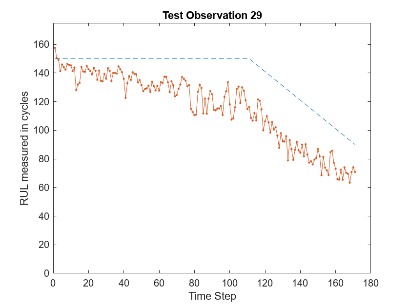
Compare Predictions with Test Data

Use a plot to compare the MEX output data with the test data.

% figure('Name', 'Standard LSTM', 'NumberTitle', 'off');
%     
% plot(YTest{idx},'--')
% hold on
% plot(YPred1,'.-')
% hold off
% 
% ylim([0 175])
% title("Test Observation " + idx)
% xlabel("Time Step")
% ylabel("RUL measured in cycles")

Clear PIL

% clear rul_lstmnet_predict_pil;

Second Approach: Generate PIL MEX Function for Stateful LSTM Network

Instead of passing the entire timeseries data all at once to predict, you can run prediction by streaming the input data segment-wise by using the predictAndUpdateState function.

The entry-point function rul_lstmnet_predict_and_update accepts a single-timestep input and processes it by using the predictAndUpdateState function. predictAndUpdateState returns a prediction for the input timestep and updates the network so that subsequent parts of the input are treated as subsequent timesteps of the same sample.

type('rul_lstmnet_predict_and_update.m')

function out = rul_lstmnet_predict_and_update(in) %#codegen

% Copyright 2019 The MathWorks, Inc. 

persistent mynet;

if isempty(mynet)
    mynet = coder.loadDeepLearningNetwork('rul_lstmnet.mat');
end

[mynet, out] = predictAndUpdateState(mynet, in);

end

Create the input type for the codegen command. Because rul_lstmnet_predict_and_update accepts a single timestep data in each call, specify the input type matrixInput to have a fixed sequence length of 1 instead of a variable sequence length.

% matrixInput = coder.typeof(double(0),[17 1]);

Run the codegen command to generate PIL based mex function rul_lstmnet_predict_and_update_pil on the host platform.

% codegen -config cfg rul_lstmnet_predict_and_update -args {matrixInput} -report

Run Generated PIL MEX Function on Test Data

% Run generated MEX function(|rul_lstmnet_predict_and_update_pil|) for each
% time step data in the inputData sequence.

% sequenceLength = size(inputData,2);
% YPred2 = zeros(1, sequenceLength);
% for i=1:sequenceLength
%     inTimeStep = inputData(:,i);
%     YPred2(:, i) = rul_lstmnet_predict_and_update_pil(inTimeStep);
% end

After you pass all timesteps, one at a time, to the rul_lstmnet_predict_and_update function, the resulting output is the same as that in the first approach in which you passed all inputs at once.

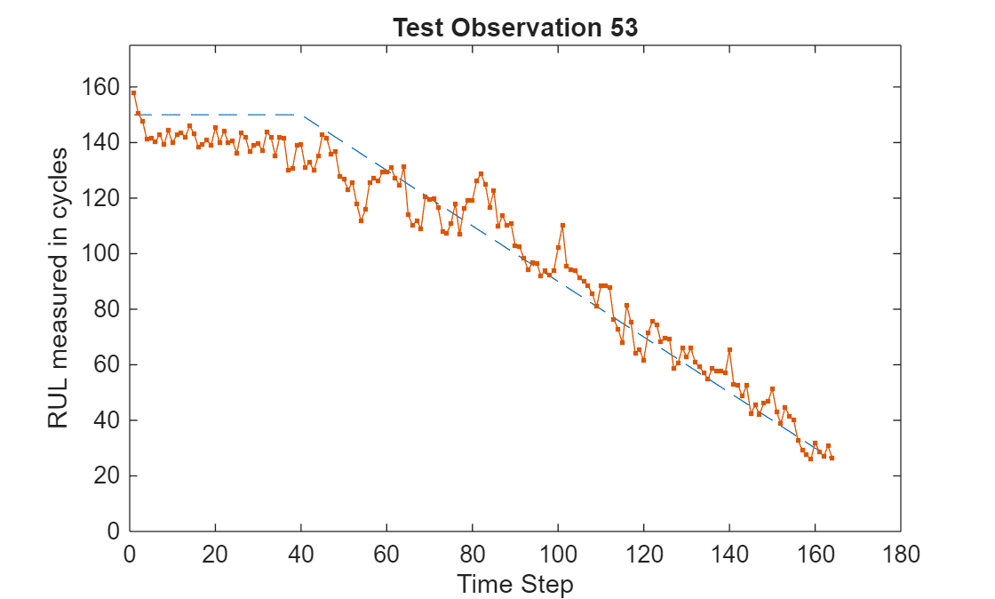
Compare Predictions with Test Data

Use a plot to compare the MEX output data with the test data.

% figure('Name', 'Statefull LSTM', 'NumberTitle', 'off');
% 
% 
% plot(YTest{idx},'--')
% hold on
% plot(YPred2,'.-')
% hold off
% 
% ylim([0 175])
% title("Test Observation " + idx)
% xlabel("Time Step")
% ylabel("RUL measured in cycles")

Clear PIL

% clear rul_lstmnet_predict_and_update_pil;

References

[1] Saxena, Abhinav, Kai Goebel, Don Simon, and Neil Eklund. "Damage propagation modeling for aircraft engine run-to-failure simulation." In Prognostics and Health Management, 2008. PHM 2008. International Conference on, pp. 1-9. IEEE, 2008.