Lidar Object Detection Using Complex-YOLO v4 Network
This example shows how to detect objects in point clouds using you only look once version 4 (YOLO v4) deep learning network. In this example, you:
Configure a dataset for training, validation, and testing of YOLO v4 object detection network. You will also perform preprocessing on how to convert point cloud to a Bird's Eye View (BEV) image.
Compute anchor boxes from the training data to use for training the YOLO v4 object detection network.
Create a YOLO v4 object detector by using the
yolov4ObjectDetectorfunction and train the detector usingtrainYOLOv4ObjectDetectorfunction.
The Complex-YOLO [1] approach is effective for lidar object detection as it directly operates on bird's-eye-view RGB maps that are transformed from the point clouds. In this example, using the Complex-YOLO approach, you train a YOLO v4 [2] network to predict both 2-D box positions and orientation in the bird's-eye-view frame. You then project the 2-D positions along with the orientation predictions back onto the point cloud to generate 3-D bounding boxes around the object of interest.
Download Lidar Data Set
This example uses a subset of the PandaSet data set that contains 2560 preprocessed organized point clouds. Each point cloud covers 360 degrees of view and is specified as a 64-by-1856 matrix. The point clouds are stored in PCD format and their corresponding ground truth data is stored in the PandaSetLidarGroundTruth.mat file. The file contains 3-D bounding box information for three classes, which are car, truck, and pedestrian. The size of the data set is 5.2 GB.
Download the PandaSet data set from the given URL using the helperDownloadPandasetData helper function, defined at the end of this example.
outputFolder = fullfile(tempdir,'Pandaset');

lidarURL = ['https://ssd.mathworks.com/supportfiles/lidar/data/' ...
            'Pandaset_LidarData.tar.gz'];

helperDownloadPandasetData(outputFolder,lidarURL);
Depending on your internet connection, the download process can take some time. The code suspends MATLAB® execution until the download process is complete. Alternatively, you can download the data set to your local disk using your web browser and extract the file. If you do so, change the outputFolder variable in the code to the location of the downloaded file. The download file contains Lidar, Cuboids, and semanticLabels folders, which contain the point clouds, cuboid label information, and semantic label information respectively.
Load Data
Create a file datastore to load the PCD files from the specified path using the pcread (Computer Vision Toolbox) function.
path = fullfile(outputFolder,'Lidar');
pcds = fileDatastore(path,'ReadFcn',@(x) pcread(x));
Load the 3-D bounding box labels of the car, truck, and pedestrian objects.
gtPath = fullfile(outputFolder,'Cuboids','PandaSetLidarGroundTruth.mat');
data = load(gtPath,'lidarGtLabels');
Labels = timetable2table(data.lidarGtLabels);
boxLabels = Labels(:,2:end);
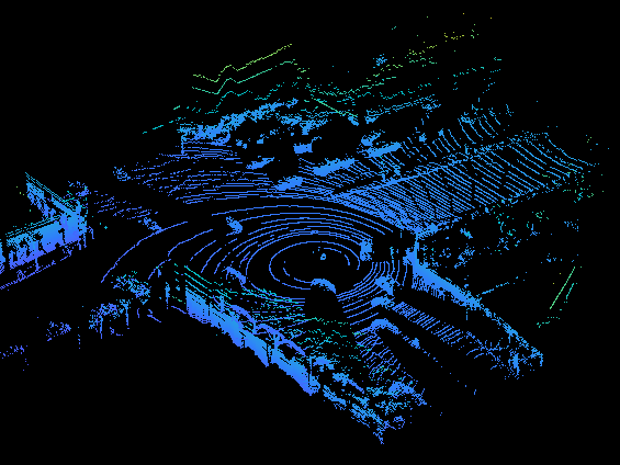
Display the full-view point cloud.
figure
ptCld = read(pcds);
ax = pcshow(ptCld.Location);
set(ax,'XLim',[-50 50],'YLim',[-40 40]);
zoom(ax,2.5);
axis off;

Create Bird's-Eye-View Image from Point Cloud Data
The PandaSet data consists of full-view point clouds. For this example, crop the full-view point clouds and convert them to a bird's-eye-view images using the standard parameters. These parameters determine the size of the input passed to the network. Selecting a smaller range of point clouds along the x-, y-, and z-axes helps you detect objects that are closer to the origin.
xMin = -25.0;
xMax = 25.0;
yMin = 0.0;
yMax = 50.0;
zMin = -7.0;
zMax = 15.0;
Define the dimensions for the bird's-eye-view image. You can set any dimensions for the bird's-eye-view image but the preprocessData helper function resizes it to network input size. For this example, the network input size is 608-by-608.
bevHeight = 608;
bevWidth = 608;
Find the grid resolution.
gridW = (yMax - yMin)/bevWidth;
gridH = (xMax - xMin)/bevHeight;
Define the grid parameters.
gridParams = {{xMin,xMax,yMin,yMax,zMin,zMax},{bevWidth,bevHeight},{gridW,gridH}};Convert the training data to bird's-eye-view images by using the transformPCtoBEV helper function, attached to this example as a supporting file. You can set writeFiles to false if your training data is already present in the outputFolder.
writeFiles = true;
if writeFiles
    transformPCtoBEV(pcds,boxLabels,gridParams,outputFolder);
end
Create Datastore Objects for Training
Use imageDatastore for loading the bird's-eye-view images.
dataPath = fullfile(outputFolder,'BEVImages');
imds = imageDatastore(dataPath);
Use boxLabelDatastore for loading the ground truth boxes.
labelPath = fullfile(outputFolder,'Cuboids','BEVGroundTruthLabels.mat');
load(labelPath,'processedLabels');
blds = boxLabelDatastore(processedLabels);
Remove the data that has no labels from the training data.
[imds,blds,pcds] = removeEmptyData(imds,blds,pcds);
Split the data set into training, validation and test sets. Select 60% of the data for training, 10% for validation, and the rest for testing the trained detector.
rng(0);
shuffledIndices = randperm(size(imds.Files,1));
idx = floor(0.6 * length(shuffledIndices));

trainingIdx = 1:idx;
validationIdx = idx+1 : (idx+1+floor(0.1*length(shuffledIndices)));
testIdx = validationIdx(end)+1 : length(shuffledIndices);
Use imageDatastore and boxLabelDatastore to create datastores for loading the image and label data during training and evaluation.
imdsTrain = subset(imds,shuffledIndices(trainingIdx));
bldsTrain = subset(blds,shuffledIndices(trainingIdx));

imdsValidation = subset(imds,shuffledIndices(validationIdx));
bldsValidation = subset(blds,shuffledIndices(validationIdx));

imdsTest = subset(imds,shuffledIndices(testIdx));
bldsTest = subset(blds,shuffledIndices(testIdx));
Combine the image and box label datastores.
trainData = combine(imdsTrain,bldsTrain);
validationData = combine(imdsValidation,bldsValidation);
testData = combine(imdsTest,bldsTest);
Use the validateInputDataComplexYOLOv4 helper function, attached to this example as a supporting file, to detect:
Samples with an invalid image format or that contain NaNs
Bounding boxes containing zeros, NaNs, Infs, or are empty
Missing or noncategorical labels.
The values of the bounding boxes must be finite and positive and cannot be NaNs. They must also be within the image boundary with a positive height and width.
validateInputDataComplexYOLOv4(trainData);
validateInputDataComplexYOLOv4(validationData);
validateInputDataComplexYOLOv4(testData);
Preprocess Training Data
Preprocess the training data to prepare for training. The preprocessData helper function, listed at the end of the example, applies the following operations to the input data.
Resize the images to the network input size.
Scale the image pixels in the range [0 1].
networkInputSize = [608 608 3];
preprocessedTrainingData = transform(trainData,@(data)preprocessData(data,networkInputSize));
Read the preprocessed training data.
data = read(preprocessedTrainingData);
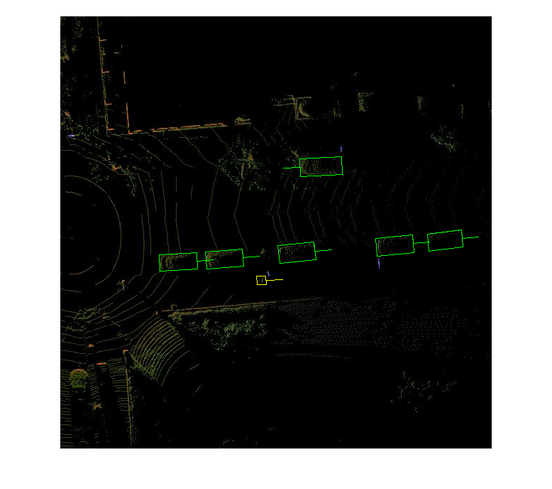
Display an image with the bounding boxes.
I = data{1,1};
bbox = data{1,2};
labels = data{1,3};
helperDisplayBoxes(I,bbox,labels);
Reset the datastore.
reset(preprocessedTrainingData);
Create a YOLOV4 Object Detection Network
Specify the name of the object class to detect.
classNames = {'Car'
              'Truck'
              'Pedestrain'};
Specify the number of anchors:
complex-yolov4-pandasetmodel— Specify 9 anchorstiny-complex-yolov4-pandasetmodel— Specify 6 anchors
For reproducibility, set the random seed. Use the estimateAnchorBoxes function to estimate anchor boxes based on the size of objects in the training data. For more information about anchor boxes, refer to "Specify Anchor Boxes" section of Getting Started with YOLO v4 (Computer Vision Toolbox).
rng(0)
numAnchors = 6;
[anchors,meanIoU] = estimateAnchorBoxes(trainData,numAnchors)
anchors = 6×2

    22    52
    10    12
    18     7
    11    16
    24    60
     9     9
meanIoU =
0.7789
Specify anchorBoxes to use in all the detection heads. anchorBoxes is a cell array of [Mx1], where M denotes the number of detection heads. Each detection head consists of a [Nx2] matrix of anchors, where N is the number of anchors to use. Select anchorBoxes for each detection head based on the feature map size. Use larger anchors at lower scale and smaller anchors at higher scale. To do so, sort the anchors with the larger anchor boxes first and assign the first three to the first detection head and the next three to the second detection head and the last three to the third detection head.
area = anchors(:, 1).*anchors(:,2);
[~,idx] = sort(area,"descend");

anchors = anchors(idx,:);
anchorBoxes = {anchors(1:3,:)
    anchors(4:6,:)
    };
Create the YOLO v4 object detector by using the yolov4ObjectDetector function. Specify the name of the pretrained YOLO v4 detection network trained on COCO dataset. Specify the class name and the estimated anchor boxes.
modelName = "tiny-yolov4-coco";
detector = yolov4ObjectDetector(modelName,classNames,anchorBoxes,InputSize=networkInputSize);
Specify Training Options
Use trainingOptions to specify network training options. Train the object detector using the Adam solver for 90 epochs with a constant learning rate 0.001. "ResetInputNormalization" should be set to false and "BatchNormalizationStatistics" should be set to "moving". Set "ValidationData" to the validation data and "ValidationFrequency" to 1000. To validate the data more often, you can reduce the “ValidationFrequency” which also increases the training time. Use "ExecutionEnvironment" to determine what hardware resources will be used to train the network. Default value for this is "auto" which selects a GPU if it is available, otherwise selects the CPU. Set "CheckpointPath" to a temporary location. This enables the saving of partially trained detectors during the training process. If training is interrupted, such as by a power outage or system failure, you can resume training from the saved checkpoint.
options = trainingOptions("adam",...
    GradientDecayFactor=0.9,...
    SquaredGradientDecayFactor=0.999,...
    InitialLearnRate=0.001,...
    LearnRateSchedule="none",...
    MiniBatchSize=4,...
    L2Regularization=0.0005,...
    MaxEpochs=50,...
    BatchNormalizationStatistics="moving",...
    DispatchInBackground=true,...
    ResetInputNormalization=false,...
    Shuffle="every-epoch",...
    VerboseFrequency=100,...
    ValidationFrequency=1000,...
    CheckpointPath=tempdir,...
    ValidationData=validationData);
Train YOLO v4 object detector.
Use the trainYOLOv4ObjectDetector function to train YOLO v4 object detector. This example is run on an NVIDIA™ Titan RTX GPU with 24 GB of memory. Training this network took approximately 6 hours using this setup. The training time will vary depending on the hardware you use. Instead of training the network, you can also use a pretrained YOLO v4 object detector.
Download the pretrained detector by using the downloadPretrainedYOLOv4Detector helper function. Set the doTraining value to false. If you want to train the detector on the augmented training data, set the doTraining value to true.
doTraining = false;

if doTraining
    [detector,info] = trainYOLOv4ObjectDetector(trainData,detector,options);
else
    % Load pretrained detector for the example.
    detector = downloadPretrainedComplexYOLOv4(modelName);
end
Evaluate Model
Computer Vision Toolbox™ provides object detector evaluation function (evaluateObjectDetection) to measure common metrics such as average precision for rotated rectangles. This example uses the average orientation similarity (AOS) metric. AOS is a metric for measuring detector performance on rotated rectangle detections. This metric provides a single number that incorporates the ability of the detector to make correct classifications (precision) and the ability of the detector to find all relevant objects (recall).
% Reset the datastore.
reset(testData)
% Run the detector on images in the test set and collect the results.
results = detect(detector,testData,'ExecutionEnvironment','cpu');

% Evaluate the object detector using the average precision metric.
metrics = evaluateObjectDetection(results,testData,'AdditionalMetrics','AOS');
metrics.ClassMetrics
ans=3×8 table
    6158    0.9466    0.9466    1×6033 double    1×6033 double    0.9050    0.9050    1×6033 double
     303    0.9151    0.9151     1×291 double     1×291 double    0.9023    0.9023     1×291 double
    3175    0.3955    0.3955    1×2496 double    1×2496 double    0.4269    0.4269    1×2496 double
Detect Objects Using Trained Complex-YOLO V4
Use the network for object detection.
% Read the datastore.
reset(testData)

% Read the BEV image from the test data.
data = read(testData);
I = data{1,1};

% Run the detector.
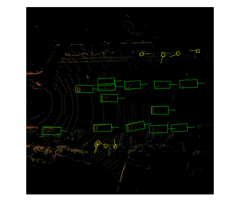
[bboxes,scores,labels] = detect(detector,I);

% Display the output.
figure
helperDisplayBoxes(I,bboxes,labels);

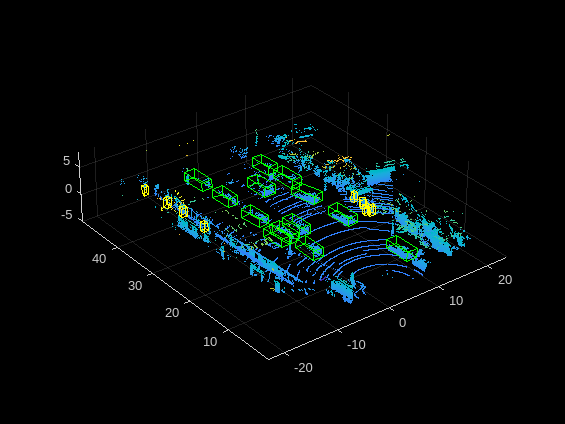
Transfer the detected boxes to a point cloud using the transferbboxToPointCloud helper function, attached to this example as a supporting file.
lidarTestData = subset(pcds,shuffledIndices(testIdx));
ptCld = read(lidarTestData);
[ptCldOut,bboxCuboid] = transferbboxToPointCloud(bboxes,gridParams,ptCld);
helperDisplayBoxes(ptCldOut,bboxCuboid,labels);

Supporting Functions
Preprocess Data
function data = preprocessData(data,targetSize)
% Resize the images and scale the pixels to between 0 and 1. Also scale the
% corresponding bounding boxes.
for ii = 1:size(data,1)
    I = data{ii,1};
    imgSize = size(I);

    % Convert an input image with a single channel to three channels.
    if numel(imgSize) < 3
        I = repmat(I,1,1,3);
    end
    bboxes = data{ii,2};

    I = im2single(imresize(I,targetSize(1:2)));
    scale = targetSize(1:2)./imgSize(1:2);
    bboxes = bboxresize(bboxes,scale);
    data(ii, 1:2) = {I,bboxes};
end
end
Utility Functions
function helperDisplayBoxes(obj,bboxes,labels)
% Display the boxes over the image and point cloud.
    figure
    if ~isa(obj,'pointCloud')
        imshow(obj)
        shape = 'rectangle';
    else
        pcshow(obj.Location);
        shape = 'cuboid';
    end
    showShape(shape,bboxes(labels=='Car',:),...
                  'Color','green','LineWidth',0.5);hold on;
    showShape(shape,bboxes(labels=='Truck',:),...
              'Color','magenta','LineWidth',0.5);
    showShape(shape,bboxes(labels=='Pedestrain',:),...
              'Color','yellow','LineWidth',0.5);
    hold off;
end

function helperDownloadPandasetData(outputFolder,lidarURL)
% Download the data set from the given URL to the output folder.
    lidarDataTarFile = fullfile(outputFolder,'Pandaset_LidarData.tar.gz');
    if ~exist(lidarDataTarFile,'file')
        mkdir(outputFolder);
        disp('Downloading PandaSet Lidar driving data (5.2 GB)...');
        websave(lidarDataTarFile,lidarURL);
        untar(lidarDataTarFile,outputFolder);
    end
    % Extract the file.
    if (~exist(fullfile(outputFolder,'Lidar'),'dir'))...
            &&(~exist(fullfile(outputFolder,'Cuboids'),'dir'))
        untar(lidarDataTarFile,outputFolder);
    end
end
References
[1] Simon, Martin, Stefan Milz, Karl Amende, and Horst-Michael Gross. "Complex-YOLO: Real-Time 3D Object Detection on Point Clouds". ArXiv:1803.06199 [Cs], 24 September 2018. https://arxiv.org/abs/1803.06199.
[2] Bochkovskiy, Alexey, Chien-Yao Wang, and Hong-Yuan Mark Liao. "YOLOv4: Optimal Speed and Accuracy of Object Detection". ArXiv:2004.10934 [Cs, Eess], 22 April 2020. https://arxiv.org/abs/2004.10934.
[3] Hesai and Scale. PandaSet. Accessed September 18, 2025. https://pandaset.org/. The PandaSet data set is provided under the CC-BY-4.0 license.
[4] Xiao, Pengchuan, Zhenlei Shao, Steven Hao, et al. “PandaSet: Advanced Sensor Suite Dataset for Autonomous Driving.” 2021 IEEE International Intelligent Transportation Systems Conference (ITSC), IEEE, September 19, 2021, 3095–101. https://doi.org/10.1109/ITSC48978.2021.9565009