Musical Instrument Classification with Joint Time-Frequency Scattering

Joint Time-Frequency Scattering

Joint time-frequency scattering (JTFS) is a modification of the wavelet scattering transform proposed in [3]. After convolving the data in time with wavelets followed by pointwise modulus nonlinearities, JTFS additionally filters the data along frequency with frequential wavelets [1],[2]. JTFS is inspired by models of the spectrotemporal receptive fields in the primary auditory cortex. Neurons in the auditory cortex exhibit ripple-like responses around specific regions in the time-frequency plane, corresponding to specific temporal and frequential modulation rates.

Consider the following example of the wavelet filter banks in a joint time-frequency scattering network.

sn = timeFrequencyScattering(EnergyCorrectFilters=false);

First, obtain and plot the Fourier transforms of the wavelet time filter banks.

[psit1,psit2,phift,timemeta] = filterbank(sn);
df = 1/size(psit1,1);
f = 0:df:1-df;
tiledlayout(2,1)
nexttile
plot(f,psit1)
grid on
ylabel("Magnitude")
title("8 Wavelets Per Octave")
nexttile
plot(f,psit2)
grid on
ylabel("Magnitude")
title("1 Wavelet Per Octave")
xlabel("Cycles/Sample")

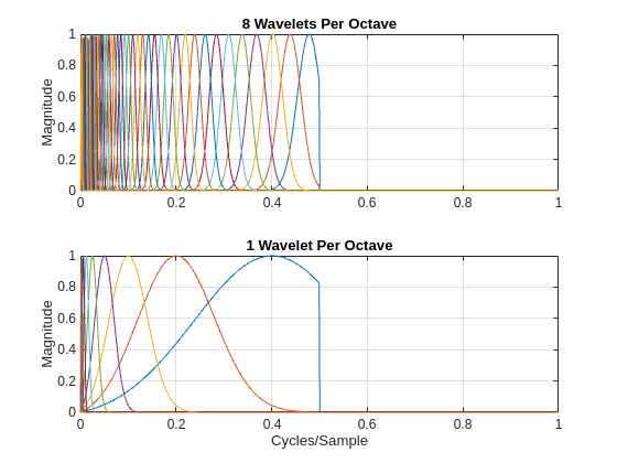
Note that the time filter banks in the JTFS network are analytic filters. Their frequency supports are restricted to only positive frequencies. Next, examine the Fourier transforms of the frequency wavelet filter banks.

[psifup,psifdown] = filterbank(sn,FilterBank="frequency");
Nf = size(psifup,1);
quef = 0:1/Nf:1-1/Nf;
figure
plot(quef,[psifup psifdown])
grid on
title("Spin-Up and Spin-Down Frequential Wavelets")
xlabel("Quefrency")
ylabel("Magnitude")

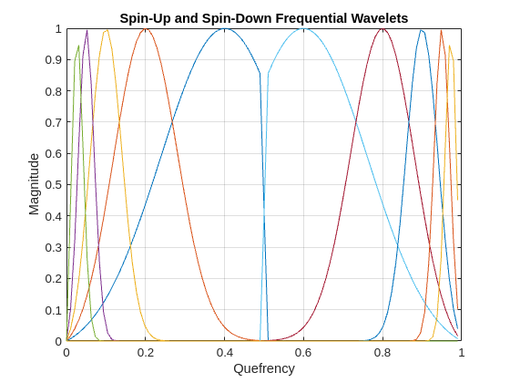
For the frequency wavelets, there are analytic (or progressive) wavelets, which are referred to as spin-up wavelets. Additionally, there are the frequency reverses (equivalently time reverses) of the spin-up wavelets, which are called spin-down wavelets. These wavelets only have support over the negative quefrencies. Similar to the lowpass filter found in wavelet time scattering, there is a lowpass frequential wavelet used in JTFS.

JTFS as Feature Extractor

As an extension of wavelet time scattering, JTFS adds sensitivity to frequency-dependent time shifts, invariance to frequency transposition, and stability against frequency and time-frequency warping.

As an illustration of how JTFS is able to separate distinct time-frequency geometries in a signal, consider the following example of a frequency-modulated signal with both exponentially increasing and decreasing chirp components.

y = echirp(10,400,2048);
z = echirp(400,10,2048);
x = y+z;

Obtain a JTFS network with time and frequency invariance scales of 32 samples and 2 quefrencies respectively. Use time quality factors of 16 and 1 wavelets per octave. Compute the JTFS transform of the signal and plot the spin-up and spin-down JTFS coefficients.

sn = timeFrequencyScattering(SignalLength=length(y),TimeInvarianceScale=32,...
    NumFrequencyOctaves=2,FrequencyInvarianceScale=2,TimeQualityFactors=16);
[outCFS,outMETA] = scatteringTransform(sn,x);
scattergram(sn,outCFS,outMETA)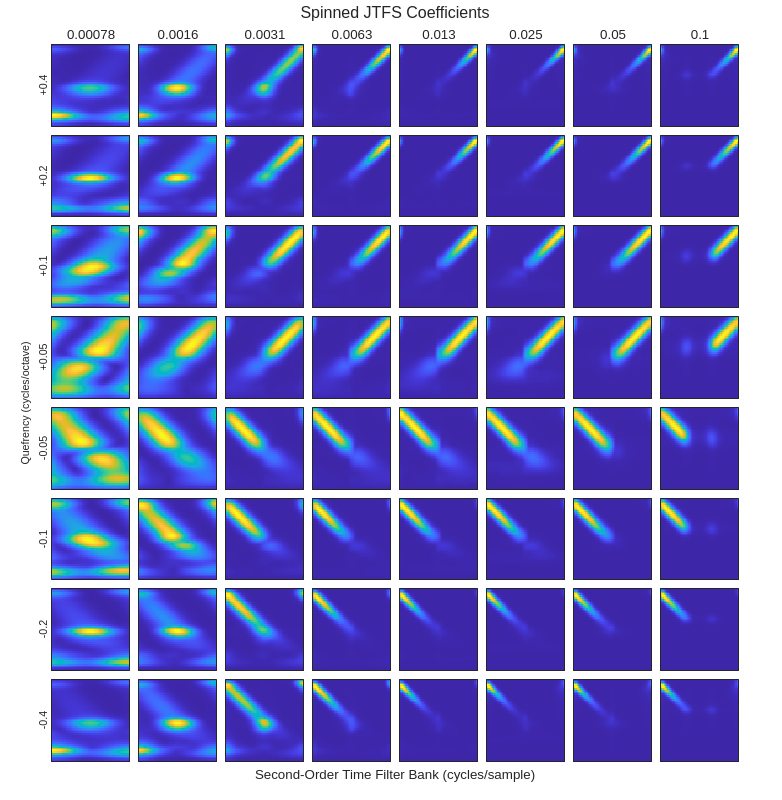

The resulting scattergram clearly demonstrates how JTFS is able to separate the exponentially increasing frequency component in the spin-up coefficients and the exponentially decreasing frequency component in the spin-down coefficients. Because wavelets in JTFS are logarithmically spaced, the chirp geometries appear linear in the JTFS transform.

Musical Instrument Data

Because of its rich time-frequency geometry, music is often a good candidate for time-frequency analysis and the additional frequency scattering in JTFS. The music data used in this example are taken from Philharmonia Sound Samples, which contains a large number of files recorded by Philharmonia musicians. This data must be obtained directly from the Philharmonia site. The license restrictions on approved use of the data are included on the linked website. This example provides a helper function, downloadPhilharmonicData, which downloads the data and writes all the required files in the proper folders. You must have an internet connection and write permission to the folder you designate as baseFolder. In this example, we use tempdir as the base folder. When fully downloaded and unzipped, the data requires about 36 MB of disk space.

baseFolder = tempdir;
downloadPhilharmonicData(baseFolder);

Downloading music samples
Unzipping all files
Unzipping bassoon files
Unzipping cello files
Unzipping clarinet files
Unzipping contrabassoon files
Unzipping double bass files
Unzipping English horn (cors anglais) files
Unzipping French horn files
Unzipping oboe files
Unzipping trombone files
Unzipping tuba files
Unzipping viola files
Unzipping violin files

The script updates you with progress as it downloads and unzips the required files. Once the data is written, create an audioDatastore to manage data access. An audioDatastore is required because the recordings are stored as MP3 files. The helper function, downloadPhilharmonicData, writes recordings belonging to separate instruments in folders named for each instrument. Use the folder name as the source of the instrument label.

dataFolder = fullfile(baseFolder,"all-samples");
ads = audioDatastore(dataFolder,IncludeSubFolders=true,...
    LabelSource="foldernames");

There are 1970 instrument examples in this subset of the data. Each recording is sampled at 44.1 kHz. The helper function selects all the files for instruments where the musician was given a fortissimo directive in recording the sample. There are 12 different instruments in the data playing various notes, including the same note across instruments. Plot the number of recordings by instrument.

numel(ads.Files)

ans = 
1970

figure
bar(unique(ads.Labels),countcats(ads.Labels))
title("Number of Recordings by Instrument")
grid on
ylabel("Number of Recordings")

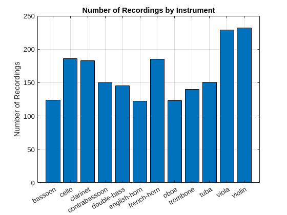
Note that the data set is imbalanced. Read through all the data once to obtain the lengths of each individual recording. If you wish to skip this step, you can move directly to the Harmonic Structure and the Power Spectrum section.

reset(ads)
audiolengths = zeros(numel(ads.Files),1);
ii = 1;
while hasdata(ads)
    audio = read(ads);
    audiolengths(ii) = length(audio);
    ii = ii+1;
end

Plot the frequency histogram of the signal lengths.

histogram(audiolengths,50)
xlabel("Length in Samples")
ylabel("Frequency")
title("Histogram of Recording Lengths")
grid on

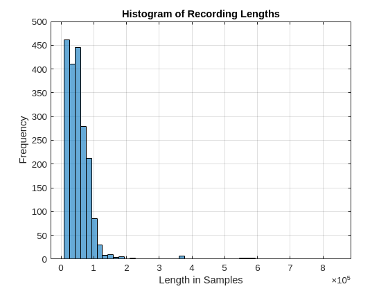
From the histogram, it is apparent that there is a positively skewed distribution of recording lengths. You can discern this from the naming convention used for the individual files which contains the approximate length in seconds. The median length for all 1970 files is 44928 samples, which is approximately 1.02 seconds of audio. The JTFS network requires a fixed input length. For relatively long signals, the JTFS implementation works most efficiently with power-of-two input lengths and setting the network TimeMaxPaddingFactor property to 0. Accordingly, use 32768 samples as the input length. Subsequently, all recordings are padding or truncated to this length in the example.

Harmonic Structure and the Power Spectrum

Read the first audio file which is a bassoon playing an A2 note.

reset(ads)
bassoonA2 = read(ads);

The note A2 on the bassoon corresponds to a fundamental frequency of 110 Hz. Examine the power spectrum of this signal to see the harmonic structure of this note on the bassoon.

L = length(bassoonA2);
[Pxx,F] = periodogram(bassoonA2,kaiser(L), L,44100,"power");
ax = newplot;
plot(ax,F,10*log10(Pxx))
xlim([0 2e3])
grid on
ax.XTick = 110:110:2e3;
xlabel("Hz")
ylabel("Power")
title("Power Spectrum of Bassoon A2")

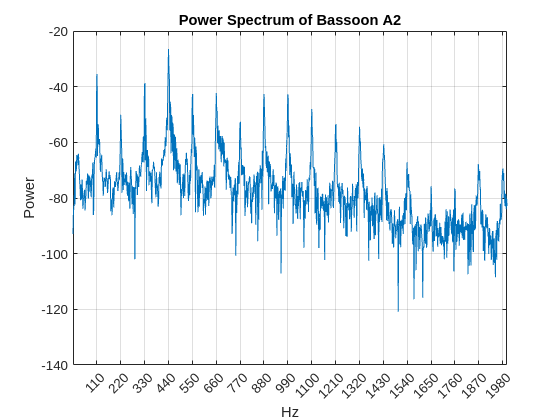
The relative power levels of the harmonics is one key factor in determining the timbre of a musical instrument. The timbre is what provides the texture to music enabling us to distinguish different instruments playing the same note. Any AI algorithm must explicitly learn these timbre distinctions to successfully classify the instrument.

Training, Validation, Test Sets and Class Weights

In subsequent sections, we use various techniques to classify instruments with deep learning networks. In preparation, split the data into 3 sets: a training set consisting of approximately 64% of the recordings, or 1260 examples, a validation set consisting of approximately 16% of the data, or 316 examples, and a test set consisting of 20% of the data, or 394 examples.

rng default
reset(ads)
[adsTrain,adsTest] = splitEachLabel(ads,0.8);
[adsTrain,adsValid] = splitEachLabel(adsTrain,0.8);

Verify that the proportions of the 12 instruments in each subset is the same.

tiledlayout(3,1)
trainlabels = adsTrain.Labels;
validlabels = adsValid.Labels;
testlabels = adsTest.Labels;
nexttile
bar(unique(trainlabels),countcats(trainlabels)./numel(trainlabels));
title("Proportion of Examples per Instrument: Training Set")
nexttile
bar(unique(validlabels),countcats(validlabels)./numel(validlabels));
title("Proportion of Examples per Instrument: Validation Set")
nexttile
bar(unique(testlabels),countcats(testlabels)./numel(testlabels));
title("Proportion of Examples per Instrument: Test Set")

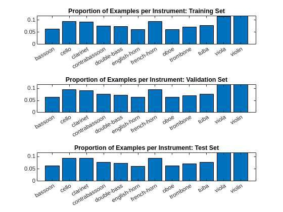
Finally, because this data set is imbalanced, compute class weights based on the inverse of the class frequency. These weights are used in all loss functions in the example.

Nc = countcats(adsTrain.Labels);
Nexamples = sum(Nc);
Nclasses = numel(unique(adsTrain.Labels));
classweights = Nexamples./(Nclasses*Nc);

Download Pretrained Models

This example provides optional pretrained model files which save you considerable time in training. If you wish to train the models, you can set doTraining to true in subsequent sections. If you wish to skip the training, download the pretrained models, MusicalInstrumentClassificationModels.zip, from the MathWorks website, https://ssd.mathworks.com/supportfiles/WA/data/MusicalInstrumentClassificationModels.zip. The models are saved under userpath. See the help for userpath if you wish to change this destination. After downloading and unzipping, the data set folder contains a text file, license.txt, with the required licensing information for the models and three .mat files, trainednetJTFS.mat, trainednetPowerSpec.mat, and trainednetSTFT.mat. The models require about 11 MB of disk space.

datasetZipFile = matlab.internal.examples.downloadSupportFile('WA','data/MusicalInstrumentClassificationModels.zip');
datasetFolder = fullfile(fileparts(datasetZipFile),'MusicalInstrumentClassificationModels');
if ~exist(datasetFolder,'dir') 
    unzip(datasetZipFile,datasetFolder);
end

Load the pretrained models for use in subsequent sections.

load(fullfile(datasetFolder,"trainednetPowerSpec.mat"));
load(fullfile(datasetFolder,"trainednetSTFT.mat"));
load(fullfile(datasetFolder,"trainednetJTFS.mat"));

1-D Convolutional Network with Power Spectra

Given that different musical instruments in this data are playing notes with the same fundamental frequency but differing harmonic structure, a reasonable assumption would be that it may be possible to separate distinct instruments solely based on harmonic structure in the frequency domain without considering the time-frequency geometry of the data. To investigate this possibility, attempt to predict the instrument based on the power spectrum using a 1-D convolutional network. The transform function, powerspectrans, included in the appendix returns the power spectrum of the instrument recording obtained with a Kaiser window and a common input length of 2^15 samples. It turns out that training a deep learning model on either the raw time series data or power spectra is inadequate for distinguishing between instruments. Specifically, the best achieved test-set accuracy was only on the order of 34%. If you wish, you can simply view the results of this section and skip to the next section, Short-Time Fourier Transform Network.

reset(adsTrain);
reset(adsValid);
reset(adsTest);
powerspectransTrain = transform(adsTrain,@(x)powerspectrans(x));
powerspectransValid = transform(adsValid,@(x)powerspectrans(x));
powerspectransTest = transform(adsTest,@(x)powerspectrans(x));

Obtain the power spectra for use in the 1-D convolutional network. If you have Parallel Computing Toolbox™, using a parallel pool greatly speeds up the computation. Set UseParallelPool to false, if you do not have the Parallel Computing Toolbox.

UseParallelPool = true;
currpool = gcp("nocreate");
if isempty(currpool)
    parpool(3);
end

Starting parallel pool (parpool) using the 'Processes' profile ...
Connected to parallel pool with 3 workers.

powerspecfeaturesTrain = readall(powerspectransTrain,UseParallel=UseParallelPool);
powerspecfeaturesValid = readall(powerspectransValid,UseParallel=UseParallelPool);
powerspecfeaturesTest = readall(powerspectransTest,UseParallel=UseParallelPool);

Reshape the individual power spectra for use in a 1-D convolutional network. Because all recordings are real-valued, we only use the one-sided power spectrum. The number of frequency bins in the one-sided power spectrum is 2^14+1.

powerspecfeaturesTrain = reshape(powerspecfeaturesTrain',2^14+1,1,[]);
powerspecfeaturesValid = reshape(powerspecfeaturesValid',2^14+1,1,[]);
powerspecfeaturesTest = reshape(powerspecfeaturesTest',2^14+1,1,[]);

Specify the training options. The same basic training options are used in each network in this example. In each case, the network with the smallest validation-set loss is used. You must set doTraining to true to train the network. This is the model trained in trainednetPowerSpec, loaded in Download Pretrained Models.

doTraining = false;
if doTraining
    numEpochs = 150; %#ok<*UNRCH>
    miniBatchSize = 128;
    initLearningRate = 0.005;
    learningRateFactor = 0.01;
    pwrspecoptions = trainingOptions("adam", ...
        InitialLearnRate=initLearningRate, ...
        LearnRateSchedule="piecewise", ...
        LearnRateDropPeriod=30, ...
        LearnRateDropFactor=learningRateFactor, ...
        MaxEpochs=numEpochs, ...
        MiniBatchSize=miniBatchSize, ...
        GradientThresholdMethod="l2norm", ...
        GradientThreshold=0.5, ...
        ValidationData = {powerspecfeaturesValid,adsValid.Labels},...
        ValidationFrequency = 100,...
        Shuffle = "every-epoch",...   
        Metrics = ["accuracy","fscore"],...
        Plots = "training-progress",...
        Verbose = false...
    ); 
    powerspectrumLayers = [
    sequenceInputLayer(1,MinLength=2^14+1,Normalization="zscore")
    convolution1dLayer(10,20,stride=4)
    batchNormalizationLayer
    reluLayer
    convolution1dLayer(8,7)
    batchNormalizationLayer
    reluLayer
    fullyConnectedLayer(100)
    dropoutLayer(0.2)
    globalAveragePooling1dLayer
    fullyConnectedLayer(12)
    softmaxLayer
    ];
    powerspecnet = trainnet(powerspecfeaturesTrain,adsTrain.Labels,powerspectrumLayers,...
        @(Y,T)crossentropy(Y,T,classweights,WeightsFormat="C"),pwrspecoptions);
end

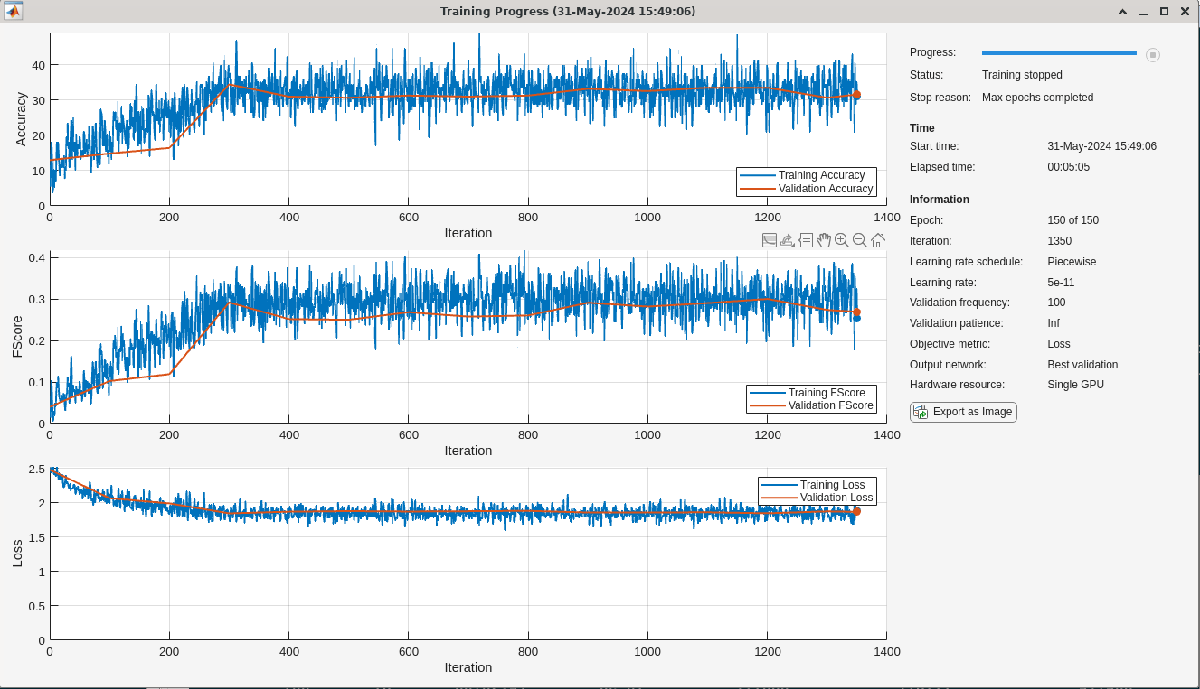
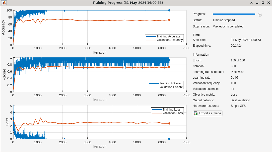
This network performs poorly as is evident from the training and validation accuracy. You can verify this by examining the accuracy on the test set.

Test the trained model on the test data. The accuracy is quite poor.

scores2TestPowerspec = minibatchpredict(trainednetPowerSpec,powerspecfeaturesTest);
predLabelsPowerspec = scores2label(scores2TestPowerspec,unique(adsTest.Labels));
sum(predLabelsPowerspec == adsTest.Labels)/numel(adsTest.Labels)

ans = 
0.3376

Short-Time Fourier Transform Network

In this section, evaluate a network that uses a time-frequency transform as features for deep learning. Specifically, this section uses the short-time Fourier transform (STFT) in a 2-D convolutional network. The example uses a differentiable STFT as a layer in the network. First, define transform functions to preprocess the audio input to a common length of 2^15 samples.

stftTransTrain = transform(adsTrain,@(x)preprocessAudio(x,transpose=true));
stftTransValid = transform(adsValid,@(x)preprocessAudio(x,transpose=true));
stftTransTest = transform(adsTest,@(x)preprocessAudio(x,transpose=true));

If you have Parallel Computing Toolbox, set UseParallelPool to true and create the training, validation, and test data. In this case, this amounts to simply preprocessing the audio and does not extract features.

UseParallelPool = true;
currpool = gcp("nocreate");
if isempty(currpool)
    parpool(3);
end
trainDataSTFT = readall(stftTransTrain,UseParallel=UseParallelPool);
validDataSTFT = readall(stftTransValid,UseParallel=UseParallelPool);
testDataSTFT = readall(stftTransTest,UseParallel=UseParallelPool);

Reshape the data in a format compatible with training a deep network.

trainDataSTFT = reshape(trainDataSTFT',2^15,1,1260);
validDataSTFT = reshape(validDataSTFT',2^15,1,316);
testDataSTFT = reshape(testDataSTFT',2^15,1,394);

If you wish to train the network, set doTraining to true. The training options and network in this section were used to train the network, trainednetSTFT, which is loaded in Download Pretrained Models. Again, the STFT is part of the network architecture. Subsequent to obtaining the STFT of each recording, a 2-D convolutional network is used for learning where convolutions are done across frequency and time.

doTraining=false;
if doTraining
    numEpochs = 150;
    miniBatchSize = 30;
    initLearningRate = 0.005;
    momentum = 0.9;
    learningRateFactor = 0.1;
    options = trainingOptions("adam", ...
        InitialLearnRate=initLearningRate, ...
        LearnRateSchedule="piecewise", ...
        LearnRateDropPeriod=30, ...
        LearnRateDropFactor=learningRateFactor, ...
        MaxEpochs=numEpochs, ...
        MiniBatchSize=miniBatchSize, ...
        GradientThresholdMethod="l2norm", ...
        GradientThreshold=0.1, ...
        Metrics = ["accuracy","fscore"],...
        Shuffle = "every-epoch",...   
        ValidationData={validDataSTFT,adsValid.Labels},...
        ValidationFrequency = 100,...
        OutputNetwork="best-validation",...
        Verbose = false,...
        Plots = "training-progress"...
        );
    numClasses = numel(unique(adsTrain.Labels));
    layersSTFT = [
        sequenceInputLayer(1,MinLength=2^15)
        stftLayer(Window=hamming(2e3),OverlapLength=700)
        convolution2dLayer([11 5],20,Name="conv2d_1",Stride=[5 1])
        batchNormalizationLayer
        reluLayer(Name="relu1")
        convolution2dLayer([9 3],20,Stride=[5 1])
        batchNormalizationLayer
        fullyConnectedLayer(100)
        dropoutLayer(0.2)
        globalAveragePooling1dLayer()
        fullyConnectedLayer(numClasses,Name="fc")
        softmaxLayer(Name="softmax")];
        trainednetSTFT = trainnet(trainDataSTFT,adsTrain.Labels,layersSTFT,@(Y,T)crossentropy(Y,T,classweights,WeightsFormat="C"),options);
end

Test the performance of the trained network on the test data.

scores2testSTFT = minibatchpredict(trainednetSTFT,testDataSTFT);
predlabelsSTFT = scores2label(scores2testSTFT,unique(adsTest.Labels));
testAccuracySTFT = sum(predlabelsSTFT == adsTest.Labels)/numel(adsTest.Labels)*100

testAccuracySTFT = 
73.0964

The test accuracy is approximately 73%. While this is a significant improvement over networks using the raw audio recordings or the power spectra, the performance is not overly impressive. Plot the confusion chart for the STFT network.

figure
confusionchart(adsTest.Labels,predlabelsSTFT,...
    ColumnSummary="column-normalized",RowSummary="row-normalized");

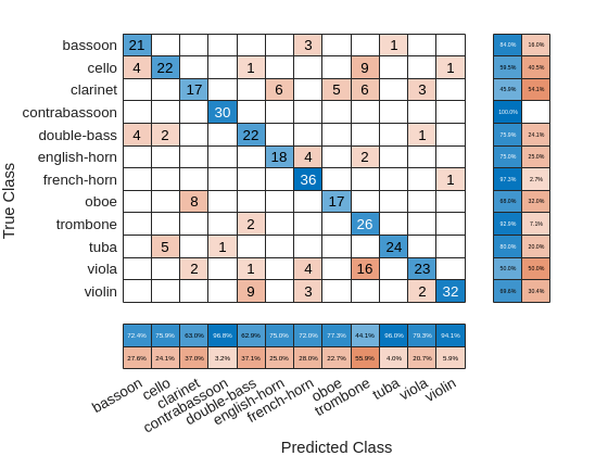
If you examine the column summaries (precision) and row summaries (recall) for each instrument, there are several instruments for which both precision and recall are quite good. However, for some instruments either precision, or recall, or both is not impressive. A good example of an instrument for which neither precision nor recall is good for this model is the clarinet.

3-D Convolutional Network with JTFS features.

The use of time-frequency features in the STFT network showed some promise. The final deep learning model in this example attempts to make that more robust by substituting JTFS features.

Create a JTFS network for a signal length of 2^15 (32768) samples. Because time-frequency geometries change rapidly in music, use relatively small values for the time and frequency invariance scales of 256 and 2, respectively. Use time quality factors of 12 and 1 wavelets per octave covering 9 and 12 octaves, respectively. Set the number of octaves covered by the frequential wavelets to 5 with 1 wavelet per octave spacing.

jtfsn = timeFrequencyScattering(signallength=2^15,...
    TimeInvarianceScale=256,...
    FrequencyInvarianceScale=2,...
    TimeQualityFactors=12,...
    NumTimeOctaves=[9 12],...
    NumFrequencyOctaves=5,...
    TimeMaxPaddingFactor=0,...
    FrequencyMaxPaddingFactor=1,...
    FilterDataType="single");

Obtain the JTFS features for use in training. If you have Parallel Computing Toolbox, use the parallel pool with 3 workers to obtain the features. Due to the relatively large number of training examples (1260) and computational complexity of the JTFS, obtaining the JTFS features requires approximately 30 minutes with the specified parallel pool. Use a transform function, jtfsFeatures, for obtaining the JTFS features. jtfsFeatures preprocesses the audio in the same manner described earlier. The JTFS transform coefficients are obtained from each preprocessed audio signal.

jtfsfeaturesTransTrain = transform(adsTrain,@(x)jtfsFeatures(x,jtfsn));
UseParallelPool = true;
currpool = gcp("nocreate");
if isempty(currpool)
    parpool(3);
end

Obtain the JTFS features for the training data.

jtfsfeatureMapsTrain = readall(jtfsfeaturesTransTrain,...
    UseParallel=UseParallelPool);

Obtain the JTFS features for the validation set. This requires approximately 7 minutes with a parallel pool using 3 workers.

jtfsfeaturesTransValid = transform(adsValid,@(x)jtfsFeatures(x,jtfsn));
jtfsfeatureMapsValid = readall(jtfsfeaturesTransValid,UseParallel=true);

Finally, obtain the JTFS features for the test set. This requires approximately 9 minutes for the parallel computation.

jtfsfeaturesTransTest = transform(adsTest,@(x)jtfsFeatures(x,jtfsn));
jtfsfeatureMapsTest = readall(jtfsfeaturesTransTest,UseParallel=true);

Permute the JTFS tensors returned by the readall operation to be in the form F-by-T-by-PB, where F is the frequency dimension of the JTFS transform, T denotes the time dimension, and PB is the product of the number of scattering paths and the batch size.

jtfsfeatureMapsTrain = permute(jtfsfeatureMapsTrain,[2 3 1]);
jtfsfeatureMapsValid = permute(jtfsfeatureMapsValid,[2 3 1]);
jtfsfeatureMapsTest = permute(jtfsfeatureMapsTest,[2 3 1]);

This example uses a 3-D convolutional architecture. The filters operate along the frequency, time, and path dimensions of the JTFS features. Contrast this with the STFT network where the filters operate along time and frequency. The 3-D convolutional network requires a channel dimension before the batch dimension. Accordingly, we reshape the JTFS feature tensors to be F-by-T-by-P-by-1-by-B.

NexamplesTrain = numel(adsTrain.Files);
NexamplesValid = numel(adsValid.Files);
NexamplesTest = numel(adsTest.Files);
Nf = size(jtfsfeatureMapsTrain,1);
Nt = size(jtfsfeatureMapsTrain,2);
Npath = size(jtfsfeatureMapsTrain,3)/NexamplesTrain;
jtfsfeatureMapsTrain = ...
    reshape(jtfsfeatureMapsTrain,Nf,Nt,Npath,1,NexamplesTrain);
jtfsfeatureMapsValid = ...
    reshape(jtfsfeatureMapsValid,Nf,Nt,Npath,1,NexamplesValid);
jtfsfeatureMapsTest = ...
    reshape(jtfsfeatureMapsTest,Nf,Nt,Npath,1,NexamplesTest);

If you wish to do the training, ensure that doTraining is true. The following 3-D convolutional network and training options were used to train the model in trainednetJTFS, which is loaded in Download Pretrained Models.

doTraining = false;
if doTraining 
    Nclasses = numel(categories(adsTrain.Labels));
    layersJTFS = [ ...
        image3dInputLayer([Nf Nt Npath 1])
        convolution3dLayer([3 8 8],4,stride=[1 4 6])
        batchNormalizationLayer
        reluLayer
        convolution3dLayer([5 5 7],3,stride=[1 2 4])
        batchNormalizationLayer
        reluLayer
        fullyConnectedLayer(250)
        reluLayer
        dropoutLayer(0.2)
        fullyConnectedLayer(Nclasses)
        softmaxLayer];
        numEpochs = 150;
        miniBatchSize = 30;
        initLearningRate = 0.005;
        learningRateFactor = 0.1;
        options = trainingOptions("adam", ...
            InitialLearnRate=initLearningRate, ...
            LearnRateSchedule="piecewise", ...
            LearnRateDropPeriod=30, ...
            LearnRateDropFactor=learningRateFactor, ...
            MaxEpochs=numEpochs, ...
            MiniBatchSize=miniBatchSize, ...
            GradientThresholdMethod="l2norm", ...
            GradientThreshold=0.5, ...
            Shuffle = "every-epoch",...            
            Metrics = ["accuracy","fscore"],...
            ValidationData={jtfsfeatureMapsValid, adsValid.Labels},...
            ValidationFrequency=100,...
            OutputNetwork="best-validation",...
            Plots = "training-progress",...
            Verbose = false...
            );
        trainednetJTFS = trainnet(jtfsfeatureMapsTrain,adsTrain.Labels, layersJTFS,...
            @(Y,T)crossentropy(Y,T,classweights,WeightsFormat="C"),options);
end

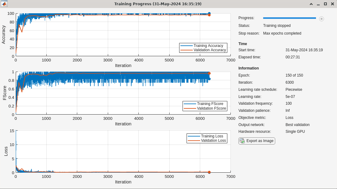
The training performance of the model is quite good. The training and validation accuracy as well as the F1 scores for both indicate good performance.

Test the trained model on the held-out test set.

scores2testJTFS = minibatchpredict(trainednetJTFS,jtfsfeatureMapsTest);
predlabelsJTFS = scores2label(scores2testJTFS,unique(adsTest.Labels));
testAccuracyJTFS = sum(predlabelsJTFS==adsTest.Labels)/numel(adsTest.Labels)*100

testAccuracyJTFS = 
93.4010

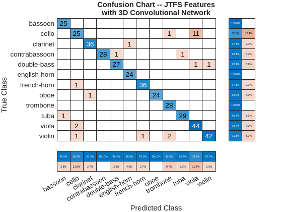
The test accuracy is approximately 93%. Plot the confusion chart for this result along with the precision and recall values for each class.

figure
confusionchart(adsTest.Labels,predlabelsJTFS,ColumnSummary="column-normalized",...
    RowSummary="row-normalized");
title({"Confusion Chart -- JTFS Features"; "with 3D Convolutional Network"})

Summary

In this example time-frequency features were paired with deep convolutional networks to classify musical instruments. In spite of the importance of harmonic structure in contributing to the timbre distinguishing distinct instruments, the use of the power spectra alone was insufficient to obtain a good classification result. Using the STFT with a 2-D convolutional architecture significantly improved the classification results obtained with the power spectra alone. However, this result was approximately 20 percentage points below what was achieved by using joint time-frequency scattering. Using the JTFS transform coefficients with a 3-D convolutional architecture achieved a test performance over 90%. While computing JTFS features increased the computational cost of feature extraction, the JTFS features provided a significant boost in accuracy.

References

[1] Anden, Joakim, Vincent Lostanlen, and Stephane Mallat. "Joint Time–Frequency Scattering." IEEE Transactions on Signal Processing 67,no. 14 (July 15, 2019): 3704–18. https://doi.org/10.1109/tsp.2019.2918992.

[2] Lostanlen, Vincent, Christian El-Hajj, Mathias Rossignol, Grégoire Lafay, Joakim Andén, and Mathieu Lagrange. "Time–Frequency Scattering Accurately Models Auditory Similarities between Instrumental Playing Techniques." EURASIP Journal on Audio, Speech, and Music Processing 2021, no. 1 (January 11, 2021). https://doi.org/10.1186/s13636-020-00187-z.

[3] Mallat, Stephane. "Group Invariant Scattering." Communications on Pure and Applied Mathematics 65, no. 10 (July 24, 2012): 1331–98. https://doi.org/10.1002/cpa.21413.

[4] Theunissen, Frederic E., Kamal Sen, and Allison J. Doupe. "Spectral-Temporal Receptive Fields of Nonlinear Auditory Neurons Obtained Using Natural Sounds." The Journal of Neuroscience 20, no. 6 (March 15, 2000): 2315–31. https://doi.org/10.1523/jneurosci.20-06-02315.2000.

[5] Wang, Changhong, Vincent Lostanlen, Emmanouil Benetos, and Elaine Chew. "Playing Technique Recognition by Joint Time–Frequency Scattering." ICASSP 2020 - 2020 IEEE International Conference on Acoustics, Speech and Signal Processing (ICASSP), May 2020. https://doi.org/10.1109/icassp40776.2020.9053474.

Appendix

The following are helper functions used in this example.

function y = echirp(f0,f1,N)
t = 0:1/1e3:(N*1e-3)-1e-3;
t1 = 2;
phi = 0;
tempVector = (f1/f0).^(t./t1);
instPhi = (t1/log(f1/f0)*f0)*(tempVector-1);
y = cos(2*pi*(instPhi+phi/360));
end

function out = preprocessAudio(audio,NVargs)
arguments
    audio
    NVargs.Transpose = false
end
audio = single(audio);
L = length(audio);
data = audio;
if L < 2^15
    data = paddata(data,2^15,side="trailing",pattern="flip");
else
    data = trimdata(data,2^15,Side="both");
end
if NVargs.Transpose
    out = data';
else
    out = data;
end
end

function out = jtfsFeatures(audio,sn)
audio = preprocessAudio(audio);
out = scatteringFeatures(sn,audio);
end

function pspec = powerspectrans(audio)
audio = single(audio);
L = length(audio);
data = audio;
if L < 2^15
    data = paddata(data,2^15,side="trailing",pattern="flip");
else
    data = trimdata(data,2^15,Side="both");
end
pspec= periodogram(data,kaiser(2^15), 2^15,[],"power");
pspec = pspec';
end