Train Neural ODE Network with Control Input

Since R2026a

This example shows how to train a neural ODE that models a swinging pendulum with torque input.

A neural ODE is a type of neural network that models the dynamics of physical systems. For physical systems with control input (physical systems that react to external factors), you can train a neural network that models the physical system using the control signals as well as the initial state of the model.

You can use neural ODEs to quickly approximate the state of physical systems.

This example trains a neural ODE model that models a swinging pendulum with torque applied.

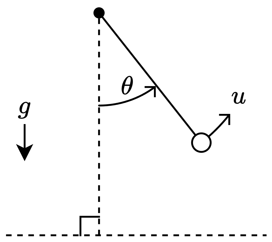
Diagram showing a swinging pendulum. There is a downwards arrow labeled g. The angle between the vertical and the pendulum is labeled theta. There is an arrow originating from the pendulum labeled u.

The system has a state $θ (t)$ , which corresponds to the angle that the pendulum makes with the vertical, the control $u (t)$ , which corresponds to the torque applied to the pendulum, and the constant acceleration $g \approx 9.81$ , which corresponds to gravity.

This diagram outlines the data flowing through the neural ODE.

Diagram showing flow of data through the neural ODE. The neural ODE has three inputs: The time interval with values [0,0.05,0.1,...,5], the initial conditions with values [theta(0), d theta(0)/dt], and control input represented by a sine wave. The output are two curves labeled "Angle" and "Angular Velocity".

Load Training Data

For this example, generate the training data using the ode45 solver. In general, you do not need to generate your own data or have the governing ODE. You can use a dataset of state measurements and corresponding control signals and train the neural network using them instead.

Neural ODEs are typically considered as ODEs of the form

$\frac{d x}{d t} = f_{p} (t, x), t \in [t_{0}, t_{1}], x (t_{0}) = x_{0} \in R^{n},$

where $f_{p} : [t_{0}, t_{1}] \times R^{n} \to R^{n}$ represents a neural network with learnable parameters $p$ . The solution $x (t)$ depends on the parameters $p$ and the initial condition $x_{0}$ . To model physical systems with control input, the neural ODE depends on additional input that corresponds to the control signal. That is, you can represent a neural ODE with control input as an ODE of the form:

$\frac{d x}{d t} = f_{p} (t, x, u), t \in [t_{0}, t_{1}], x (t_{0}) = x_{0} \in R^{n},$

where $u : [t_{0}, t_{1}] \to R^{n}$ is a control signal that controls a component in the physical system.

Training a neural ODE with control input requires a dataset of observations that correspond to $x_{0}$ , $x (t)$ , and $u (t)$ over a fixed set of time steps in the interval $[t_{0}, t_{1}]$ .

In this example, $x (t) = [θ (t), d θ (t) / d t]$ corresponds to the state of the physical system and $u (t)$ corresponds to the torque applied to the pendulum. For simplicity, define the angular momentum $ω = d θ / d t$ . Using Newtonian mechanics, the second-order ODE for $θ$ is

$\frac{d ω}{d t} = - g \sin θ + u$ .

Define the pendulum ODE function that evaluates the physical system state. The pendulumODE function takes the values for $t$ , $x$ , and $u$ as input. The function returns Y, where the first row of Y is the angular velocity $ω$ and the second row of Y is $d ω / d t$ .

function Y = pendulumODE(t,x,u)

g = 9.81;
Y = [x(2,:); -g*sin(x(1,:)) + u(t)];

end

Generate the data for 500 observations. Generate these arrays:

tspan — Vector of time steps that represent the interval of integration. Use a vector over the time interval [0,1] with step sizes of 0.1.
U — Cell array of control signal inputs. Use sine waves of varying phase.
X0 — Cell array of initial conditions. Use the first time step of solutions given by the ode45 solver with random initial conditions.
targets — Cell array of targets. Use the remaining time steps of the solutions given by the ode45 solver.

numObservations = 500;
tspan = 0:0.1:1;

controlSize = 1;
stateSize = 2;

numTimeSteps = numel(tspan);

UTrain = zeros(numTimeSteps,controlSize,numObservations);
X0Train = zeros(numObservations,stateSize);
targetsTrain = zeros(numTimeSteps-1,stateSize,numObservations);

for n = 1:numObservations
    UTrain(:,:,n) = 2*sin(2*pi*(tspan + rand))';

    u = griddedInterpolant(tspan,UTrain(:,:,n));
    odeFcn = @(t,x) pendulumODE(t,x,u);

    theta0 = pi*(2*rand - 1);
    [~,X] = ode45(odeFcn, tspan, [theta0 0]);

    X0Train(n,:) = X(1,:);
    targetsTrain(:,:,n) = X(2:end,:);
end

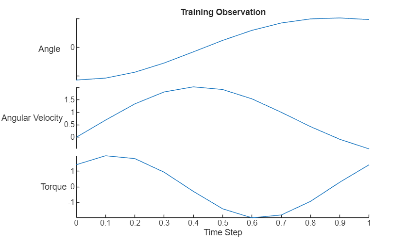
Visualize the first training observation in a plot.

data = [[X0Train(1,:); targetsTrain(:,:,1)] UTrain(:,1)];
figure
stackedplot(tspan,data,DisplayLabels=["Angle" "Angular Velocity" "Torque"]);
xlabel("Time Step")
title("Training Observation")

Define Neural Network Architecture

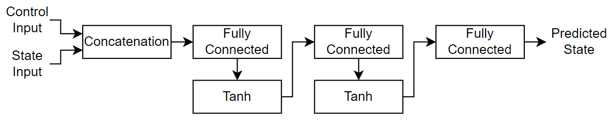
For the neural ODE network, create a multilayer perceptron (MLP) that takes the physical state and control signal as input and outputs. For the body of the network, use two fully connected layers with an output size of 20. For the network output, use a fully connected layer with an output size that matches the size of the physical system state size.

Diagram of neural network. The two inputs "Control Input" and "State Input" are passed to a concetenation layer. Then, there are three fully connected layers with tanh layers between them. The output of the last fully connected layer is labeled "Predicted State"

hiddenSize = 20;

net = dlnetwork;

layers = [
    featureInputLayer(controlSize)
    concatenationLayer(1,2,Name="cat")
    fullyConnectedLayer(hiddenSize)
    tanhLayer
    fullyConnectedLayer(hiddenSize)
    tanhLayer
    fullyConnectedLayer(stateSize)];

net = addLayers(net,layers);

layer = featureInputLayer(stateSize,Name="in_state");
net = addLayers(net,layer);
net = connectLayers(net,"in_state","cat/in2");

Initialize the neural network for training with a custom training loop.

net = initialize(net);

Define Neural ODE Function

The deep learning model in this example evaluates the neural ODE operation using the dlode45 function. Define the ODE function for the dlode45 function to evaluate.

The function odeModel takes the time value t, the state X, and a structure of parameters p as input. The parameters structure contains the interval of integration tspan, the control input u, and the ODE neural network net. The function returns the derivative of the state with respect to the time t.

The dlode45 function evaluates the ODE function at many additional intermediate time steps in the interval of integration. To evaluate the ODE function with values of $u$ for these additional time steps, the ODE function interpolates the values of $u$ using the interp1 function. To ensure that the function does not return NaN values for queries outside the interval of integration, the function thresholds these values.

function dXdt = odeModel(t,X,p)

tspan = p.tspan;
U = p.U;
net = p.net;

Ut = interp1(tspan,U,min(t,tspan(end)));

Ut = dlarray(Ut,"CB");
dXdt = forward(net,Ut,X);

end

Define Model Function

Define the model function that returns the model predictions. The function model takes the ODE neural network, the interval of integration tspan, the control input u, and the initial conditions X0 as input. The function returns the model predictions X that correspond to the predicted state of the physical system.

function X = model(net,tspan,U,X0)

p = struct;
p.tspan = tspan;
p.U = U;
p.net = net;

X = dlode45(@odeModel,tspan,X0,p, ...
    GradientMode="adjoint-seminorm");

end

Define Model Loss Function

Define the model loss function that returns the model loss and the gradients of the loss with respect to the learnable parameters of the model. The function modelLoss takes the ODE neural network, the interval of integration tspan, the control input u, the initial conditions X0, and the targets as input.

function [loss,gradients] = modelLoss(net,tspan,u,X0,targets)

X = model(net,tspan,u,X0);

loss = l2loss(X,targets);

gradients = dlgradient(loss,net.Learnables);

end

Define Training Step Function

To effectively utilize deep learning function acceleration that accelerates evaluating the model loss and the update step of the learnable parameters, define the training step function that evaluates the model loss, gradients, and the solver update step.

The trainingStep function takes the ODE neural network, the interval of integration tspan, the control input u, the initial conditions X0, the targets, and the solver parameters as input. The function returns the model loss, gradients, and updated solver parameters.

function [loss,net,avgG,avgSqG] = trainingStep(net,tspan,u,X0,targets, ...
    avgG,avgSqG,iteration,learningRate)

[loss,gradients] = modelLoss(net,tspan,u,X0,targets);

[net,avgG,avgSqG] = adamupdate(net,gradients, ...
    avgG,avgSqG,iteration,learningRate);

end

This function fully supports acceleration using the dlaccelerate function.

Specify Training Options

Train for 1000 epochs with a mini-batch size of 250.

numEpochs = 2000;
miniBatchSize = 250;
learningRate = 0.0005;

Train Neural Network

Train the neural network using a custom training loop.

Create array datastores that read mini-batches of the training data.

adsUTrain = arrayDatastore(UTrain, ...
    ReadSize=miniBatchSize, ...
    IterationDimension=3);

adsX0Train = arrayDatastore(X0Train, ...
    ReadSize=miniBatchSize);

adsTargetsTrain = arrayDatastore(targetsTrain, ...
    ReadSize=miniBatchSize, ...
    IterationDimension=3);

Combine these datastores into a single datastore that returns mini-batches of the control inputs, initial conditions, and the targets.

cdsTrain = combine(adsUTrain,adsX0Train,adsTargetsTrain);

Create a minibatchqueue object that processes and manages the mini-batches of data during training.

Use the mini-batch size specified in the training options.
Specify that the outputs have the formats "" (unformatted), "BC" (batch, channel), and "TCB" (time, channel, batch). By default, the minibatchqueue object converts the data to dlarray objects with underlying type single.
Because the data and ODE model operations are not well suited for GPU computation, the CPU is better suited for training. Set the OutputEnvironment argument to "cpu".

mbq = minibatchqueue(cdsTrain,3, ...
    MiniBatchSize=miniBatchSize, ...
    MiniBatchFormat=["" "BC" "TCB"], ...
    OutputEnvironment="cpu");

Initialize the parameters for the Adam solver and training loop.

avgG = [];
avgSqG = [];
iteration = 0;
epoch = 0;

To speed up training, use the dlaccelerate function to create an AcceleratedFunction object that automatically optimizes, caches, and reuses the traces. For more information, see Deep Learning Function Acceleration. Because the solver update step is part of the training function, and because it depends on the iteration number, convert the iteration number and learning rate to a dlarray object.

trainingStepFcn = dlaccelerate(@trainingStep);
tspan = dlarray(tspan);
iteration = dlarray(iteration);
learningRate = dlarray(learningRate);

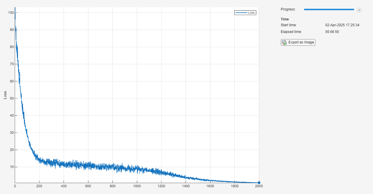
Monitor the training using a training progress monitor. Initialize a monitor that monitors the loss using the trainingProgressMonitor function. Because the timer starts when you create the monitor object, make sure that you create the object close to the training loop.

monitor = trainingProgressMonitor(Metrics="Loss");

Train the model using a custom training loop. For each epoch, shuffle the data and loop over the mini-batches of data. For each mini-batch, evaluate the training step function that updates the model learnable parameters. At the end of each epoch, update the training progress monitor.

while epoch < numEpochs && ~monitor.Stop
    epoch = epoch + 1;

    shuffle(mbq)

    while hasdata(mbq) && ~monitor.Stop
        iteration = iteration + 1;

        [UBatch,X0Batch,targetsBatch] = next(mbq);

        [loss,net,avgG,avgSqG] = dlfeval(trainingStepFcn, ...
            net,tspan,UBatch,X0Batch,targetsBatch,avgG,avgSqG,iteration,learningRate);
    end

    recordMetrics(monitor,epoch,Loss=loss);
    monitor.Progress = 100*epoch/numEpochs;
end

Make Predictions Using Unseen Data

Make predictions using a new unseen control signal for a longer time span.

Generate some input data:

Specify an interval of integration of [0,5] with a step size of 0.05.
Use a sine wave as the control input.
Use some random values for the initial conditions.

tspanNew = 0:0.05:5;

UNew = 2*sin(2*pi*(tspanNew + rand))';
X0New = [pi*(2*rand - 1); 0];

Convert the data to dlarray and make predictions using the model function.

UNew = dlarray(UNew);
tspanNew = dlarray(tspanNew);
X0New = dlarray(X0New,"CB");

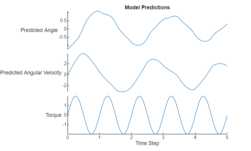
XNew = model(net,tspanNew,UNew,X0New);

Visualize the predictions in a plot.

tspanNew = extractdata(tspanNew);
UNew = extractdata(UNew);
XNew = extractdata(XNew);
X0New = extractdata(X0New);

XNew = permute(XNew,[3 1 2]);
X0New = X0New';

data = [[X0New; XNew] UNew];

figure
stackedplot(tspanNew,data, ...
    DisplayLabels=["Predicted Angle" "Predicted Angular Velocity" "Torque"]);
xlabel("Time Step")
title("Model Predictions")

Compare Results With ODE Solver

Compare the predictions with the output of the ode45 solver.

Calculate the targets using the ode45 function.

u = griddedInterpolant(tspanNew,UNew);
odeFcn = @(t,x) pendulumODE(t,x,u);
[~,targetsNew] = ode45(odeFcn, tspanNew, X0New);

Visualize the difference between the model predictions and the ODE solver output in a plot.

figure
tiledlayout
nexttile
plot(tspanNew, targetsNew(:,1));

hold on
plot(tspanNew(2:end), XNew(:,1),"--");

title("Comparison With ODE Solver")
ylabel("Angle")
legend(["ODE45 Solver" "Neural ODE"])

nexttile
plot(tspanNew, targetsNew(:,2));
hold on
plot(tspanNew(2:end), XNew(:,2),"--");
ylabel("Angular Velocity");
xlabel("Time Step")

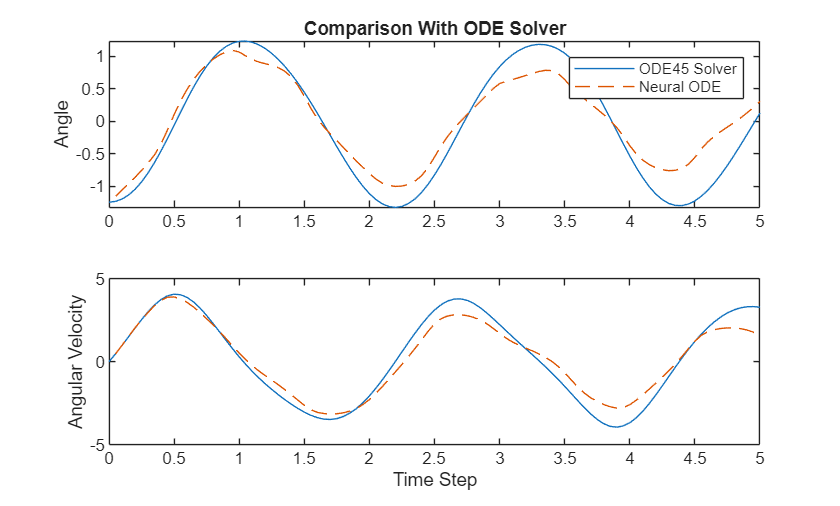
The plot shows how well the neural ODE can approximate the solutions of the ODE. Depending on the task and hardware used, the model predictions can be quicker to evaluate than computing the solutions numerically.