Adapt Pretrained Audio Network for New Data Using Deep Network Designer
This example shows how to interactively adapt a pretrained network to classify new audio signals using Deep Network Designer.
Transfer learning is commonly used in deep learning applications. You can take a pretrained network and use it as a starting point to learn a new task. Fine-tuning a network with transfer learning is usually much faster and easier than training a network with randomly initialized weights from scratch. You can quickly transfer learned features to a new task using a smaller number of training signals.
This example retrains YAMNet, a pretrained convolutional neural network, to classify a new set of audio signals.
Load Data
Download and unzip the air compressor data set [1]. This data set consists of recordings from air compressors in a healthy state or one of seven faulty states.
zipFile = matlab.internal.examples.downloadSupportFile('audio','AirCompressorDataset/AirCompressorDataset.zip');
dataFolder = fileparts(zipFile);
unzip(zipFile,dataFolder);
Create an audioDatastore object to manage the data.
ads = audioDatastore(dataFolder,IncludeSubfolders=true,LabelSource="foldernames");Extract the class names.
classNames = categories(ads.Labels);
Split the data into training, validation, and test sets using the splitEachLabel function.
[adsTrain,adsValidation,adsTest] = splitEachLabel(ads,0.7,0.2,0.1,"randomized");Use the transform function to preprocess the data using the function audioPreprocess, found at the end of this example. For each signal:
Use
yamnetPreprocess(Audio Toolbox) to generate mel spectrograms suitable for training using YAMNet. Each audio signal produces multiple spectrograms.Duplicate the class label for each of the spectrograms.
tdsTrain = transform(adsTrain,@audioPreprocess,IncludeInfo=true);
tdsValidation = transform(adsValidation,@audioPreprocess,IncludeInfo=true);
tdsTest = transform(adsTest,@audioPreprocess,IncludeInfo=true);
Select Pretrained Network
Prepare and train the network interactively using Deep Network Designer. To open Deep Network Designer, on the Apps tab, under Machine Learning and Deep Learning, click the app icon. Alternatively, you can open the app from the command line.
deepNetworkDesigner
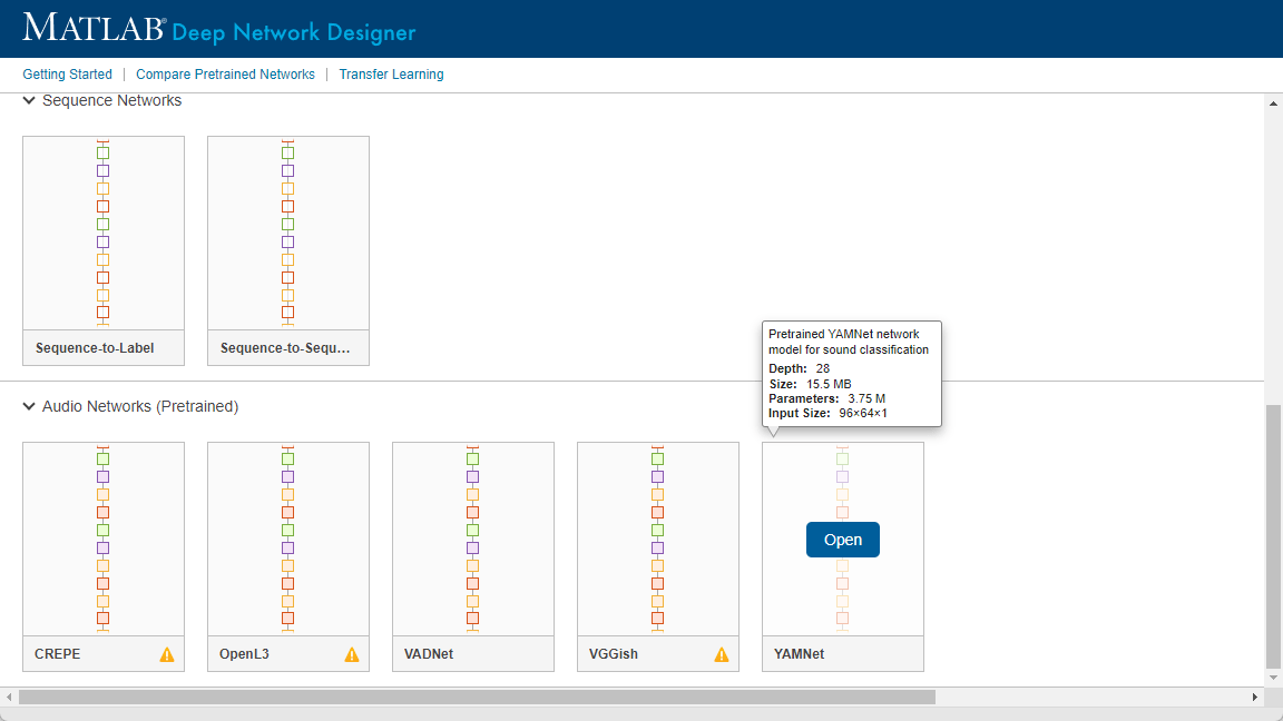
Deep Network Designer provides a selection of pretrained audio classification networks. These models require both Audio Toolbox™ and Deep Learning Toolbox™.

Under Audio Networks, select YAMNet from the list of pretrained networks and click Open. If the Audio Toolbox model for YAMNet is not installed, click Install instead. Deep Network Designer provides a link to the location of the network weights. Unzip the file to a location on the MATLAB path. Now close the Deep Network Designer Start Page and reopen it. When the network is correctly installed and on the path, you can click the Open button on YAMNet. The YAMNet model can classify audio into one of 521 sound categories. For more information, see yamnet (Audio Toolbox).
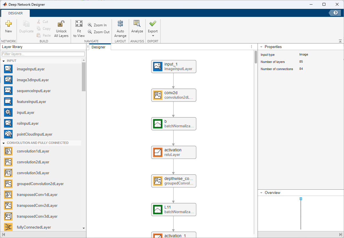
Deep Network Designer displays a zoomed-out view of the whole network in the Designer pane. To zoom in with the mouse, use Ctrl+scroll wheel. To pan, use the arrow keys, or hold down the scroll wheel and drag the mouse. Select a layer to view its properties. Clear all layers to view the network summary in the Properties pane.

Prepare Network for Transfer Learning
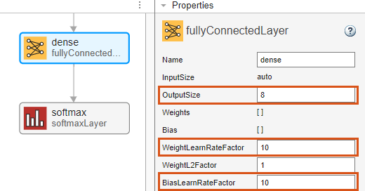
To use a pretrained network for transfer learning, you must change the number of classes to match your new data set. First, find the last learnable layer in the network. For YAMNet, the last learnable layer is the last fully connected layer, dense. At the bottom of the Properties pane, click Unlock Layer. In the warning dialog that appears, click Unlock Anyway. This unlocks the layer properties so that you can adapt them to your new task.
Before R2023b: To edit the layer properties, you must replace the layers instead of unlocking them.
The OutputSize property defines the number of classes for classification problems. Change OutputSize to the number of classes in the new data, in this example, 8.
Change the learning rates so that learning is faster in the new layer than in the transferred layers by setting WeightLearnRateFactor and BiasLearnRateFactor to 10.

To check that the network is ready for training, click Analyze. If the Deep Learning Network Analyzer reports zero errors, then the edited network is ready for training. To export the network, click Export. The app saves the network as the variable net_1.
Select Training Options
Specify the training options. Choosing among the options requires empirical analysis. To explore different training option configurations by running experiments, you can use the Experiment Manager app.
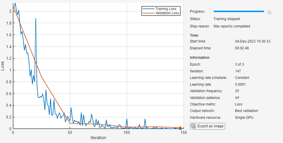
Train using the Adam optimizer.
Set the initial learning rate to a small value to slow down learning in the transferred layers. In combination with the increased learning rate factors for the fully connected layer, learning is now fast only in the new layers and slower in the other layers.
Train for 3 epochs.
To validate the network performance at regular intervals during training, specify validation data. Validate the network every 25 iterations.
Display the training progress in a plot and monitor the root mean squared error.
Disable the verbose output.
options = trainingOptions("adam", ...
    InitialLearnRate=0.0001, ...
    MaxEpochs=3, ...
    ValidationData=tdsValidation, ...
    ValidationFrequency=25, ...
    Plots="training-progress", ...
    Verbose=0);
Train Network
Train the neural network using the trainnet function. For classification tasks, use cross-entropy loss. By default, the trainnet function uses a GPU if one is available. Using a GPU requires a Parallel Computing Toolbox™ license and a supported GPU device. For information on supported devices, see GPU Computing Requirements (Parallel Computing Toolbox). Otherwise, the trainnet function uses the CPU. To specify the execution environment, use the ExecutionEnvironment training option.
net = trainnet(tdsTrain,net_1,"crossentropy",options);
Test Network
Make predictions using the minibatchpredict function. By default, the minibatchpredict function uses a GPU if one is available.
data = readall(tdsTest);
T = [data{:,2}];

scores = minibatchpredict(net,tdsTest);
Y = scores2label(scores,classNames);
accuracy = sum(Y == T')/numel(T)
accuracy = 0.9898
Supporting Function
The function audioPreprocess uses yamnetPreprocess (Audio Toolbox) to generate mel spectrograms from audioIn that you can feed to the YAMNet pretrained network. Each input signal generates multiple spectrograms, so the labels must be duplicated to create a one-to-one correspondence with the spectrograms.
function [data,info] = audioPreprocess(audioIn,info)
class = info.Label;
fs = info.SampleRate;
features = yamnetPreprocess(audioIn,fs);

numSpectrograms = size(features,4);

data = cell(numSpectrograms,2);
for index = 1:numSpectrograms
    data{index,1} = features(:,:,:,index);
    data{index,2} = class;
end
end
References
[1] Verma, Nishchal K., Rahul Kumar Sevakula, Sonal Dixit, and Al Salour. “Intelligent Condition Based Monitoring Using Acoustic Signals for Air Compressors.” IEEE Transactions on Reliability 65, no. 1 (March 2016): 291–309. https://doi.org/10.1109/TR.2015.2459684.
See Also
Deep Network Designer | yamnet