advance
Advance driving scenario simulation by one time step
Description
isRunning = advance(scenario)SampleTime property of the input drivingScenario object,
scenario. The function returns the status,
isRunning, of the simulation.
Examples
Create a driving scenario. Use the default sample time of 0.01 second.
scenario = drivingScenario;
Add a straight, 30-meter road to the scenario. The road has two lanes.
roadCenters = [0 0; 30 0];
road(scenario,roadCenters,'Lanes',lanespec(2));
Add a vehicle that travels in the left lane at a constant speed of 30 meters per second. Plot the scenario before running the simulation.
v = vehicle(scenario,'ClassID',1);
waypoints = [5 2; 25 2];
speed = 30; % m/s
smoothTrajectory(v,waypoints,speed)

plot(scenario)

Call the advance function in a loop to advance the simulation one time step at a time. Pause every 0.01 second to observe the motion of the vehicle on the plot.
while advance(scenario)
    pause(0.01)
end

Create a driving scenario and show how target outlines change as the simulation advances.
Create a driving scenario consisting of two intersecting straight roads. The first road segment is 45 meters long. The second straight road is 32 meters long with jersey barriers along both its edges, and intersects the first road. A car traveling at 12.0 meters per second along the first road approaches a running pedestrian crossing the intersection at 2.0 meters per second.
scenario = drivingScenario('SampleTime',0.1,'StopTime',1);
road1 = road(scenario,[-10 0 0; 45 -20 0]);
road2 = road(scenario,[-10 -10 0; 35 10 0]);
barrier(scenario,road1)
barrier(scenario,road1,'RoadEdge','left')
ped = actor(scenario,'ClassID',4,'Length',0.4,'Width',0.6,'Height',1.7);
car = vehicle(scenario,'ClassID',1);
pedspeed = 2.0;
carspeed = 12.0;
smoothTrajectory(ped,[15 -3 0; 15 3 0],pedspeed);
smoothTrajectory(car,[-10 -10 0; 35 10 0],carspeed);
Create an ego-centric chase plot for the vehicle.
chasePlot(car,'Centerline','on')
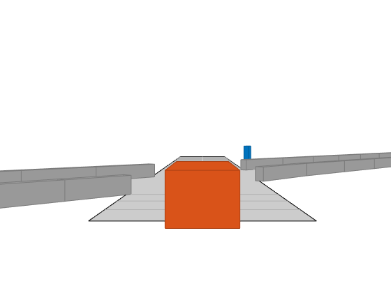
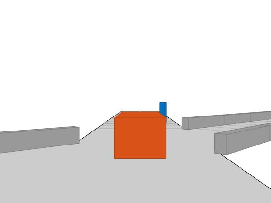
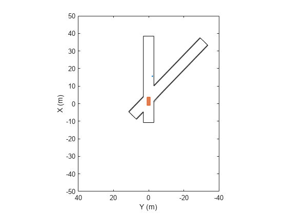
Create an empty bird's-eye plot and add an outline plotter and lane boundary plotter. Then, run the simulation. At each simulation step:
Update the chase plot to display the road boundaries and target outlines.
Update the bird's-eye plot to display the updated road boundaries and target outlines. The plot perspective is always with respect to the ego vehicle.
bepPlot = birdsEyePlot('XLim',[-50 50],'YLim',[-40 40]);
outlineplotter = outlinePlotter(bepPlot);
laneplotter = laneBoundaryPlotter(bepPlot);
legend('off')

while advance(scenario)
    rb = roadBoundaries(car);
    [position,yaw,length,width,originOffset,color] = targetOutlines(car);
    [bposition,byaw,blength,bwidth,boriginOffset,bcolor,barrierSegments] = targetOutlines(car,'Barriers');
    plotLaneBoundary(laneplotter,rb)
    plotOutline(outlineplotter,position,yaw,length,width, ...
        'OriginOffset',originOffset,'Color',color)
    plotBarrierOutline(outlineplotter,barrierSegments,bposition,byaw,blength,bwidth, ...
        'OriginOffset',boriginOffset,'Color',bcolor)
    pause(0.01)
end
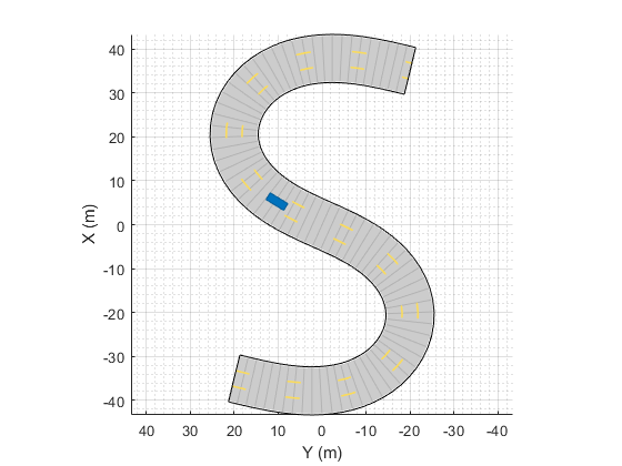
Simulate a driving scenario with one car traveling on an S-curve. Create and plot the lane boundaries.
Create the driving scenario with one road having an S-curve.
scenario = drivingScenario('StopTime',3);
roadcenters = [-35 20 0; -20 -20 0; 0 0 0; 20 20 0; 35 -20 0];
Create the lanes and add them to the road.
lm = [laneMarking('Solid','Color','w'); ...
    laneMarking('Dashed','Color','y'); ...
    laneMarking('Dashed','Color','y'); ...
    laneMarking('Solid','Color','w')];
ls = lanespec(3,'Marking',lm);
road(scenario,roadcenters,'Lanes',ls);
Add an ego vehicle and specify its trajectory from its waypoints. By default, the car travels at a speed of 30 meters per second.
car = vehicle(scenario, ...
    'ClassID',1, ...
    'Position',[-35 20 0]);
waypoints = [-35 20 0; -20 -20 0; 0 0 0; 20 20 0; 35 -20 0];
smoothTrajectory(car,waypoints);
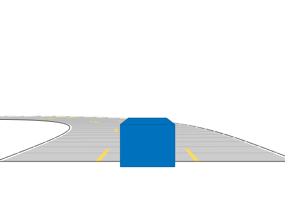
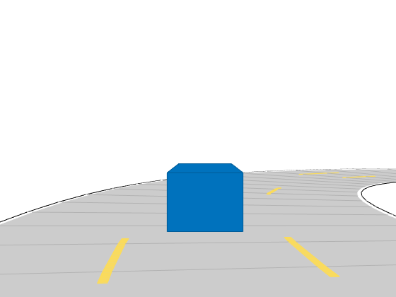
Plot the scenario and corresponding chase plot.
plot(scenario)
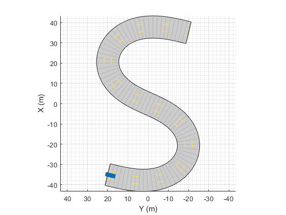
chasePlot(car)
Run the simulation loop.
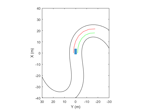
Initialize a bird's-eye plot and create an outline plotter, left-lane and right-lane boundary plotters, and a road boundary plotter.
Obtain the road boundaries and rectangular outlines.
Obtain the lane boundaries to the left and right of the vehicle.
Advance the simulation and update the plotters.
bep = birdsEyePlot('XLim',[-40 40],'YLim',[-30 30]);
olPlotter = outlinePlotter(bep);
lblPlotter = laneBoundaryPlotter(bep,'Color','r','LineStyle','-');
lbrPlotter = laneBoundaryPlotter(bep,'Color','g','LineStyle','-');
rbsEdgePlotter = laneBoundaryPlotter(bep);
legend('off');
while advance(scenario)
    rbs = roadBoundaries(car);
    [position,yaw,length,width,originOffset,color] = targetOutlines(car);
    lb = laneBoundaries(car,'XDistance',0:5:30,'LocationType','Center', ...
        'AllBoundaries',false);
    plotLaneBoundary(rbsEdgePlotter,rbs)
    plotLaneBoundary(lblPlotter,{lb(1).Coordinates})
    plotLaneBoundary(lbrPlotter,{lb(2).Coordinates})
    plotOutline(olPlotter,position,yaw,length,width, ...
        'OriginOffset',originOffset,'Color',color)
end
Input Arguments
Driving scenario, specified as a drivingScenario object.
Output Arguments
Run state of the simulation, returned as logical 1
(true) or 0
(false).
If
isRunningis1, the simulation is running.If
isRunningis0, the simulation has stopped running.
A simulation runs until at least one of these conditions are met:
The simulation time exceeds the simulation stop time. To specify the stop time, use the
StopTimeproperty ofscenario.Any actor or vehicle reaches the end of its assigned trajectory. The assigned trajectory is specified by the most recent call to the trajectory function.
The advance function updates actors
and vehicles only if they have an assigned trajectory. To update actors and
vehicles that have no assigned trajectories, you can set the
Position, Velocity,
Roll, Pitch,
Yaw, or AngularVelocity
properties at any time during simulation.
Version History
Introduced in R2017a
MATLAB Command
You clicked a link that corresponds to this MATLAB command:
Run the command by entering it in the MATLAB Command Window. Web browsers do not support MATLAB commands.
选择网站
选择网站以获取翻译的可用内容,以及查看当地活动和优惠。根据您的位置,我们建议您选择:。
您也可以从以下列表中选择网站:
如何获得最佳网站性能
选择中国网站(中文或英文)以获得最佳网站性能。其他 MathWorks 国家/地区网站并未针对您所在位置的访问进行优化。
美洲
- América Latina (Español)
- Canada (English)
- United States (English)
欧洲
- Belgium (English)
- Denmark (English)
- Deutschland (Deutsch)
- España (Español)
- Finland (English)
- France (Français)
- Ireland (English)
- Italia (Italiano)
- Luxembourg (English)
- Netherlands (English)
- Norway (English)
- Österreich (Deutsch)
- Portugal (English)
- Sweden (English)
- Switzerland
- United Kingdom (English)