Highway Trajectory Planning Using Frenet Reference Path

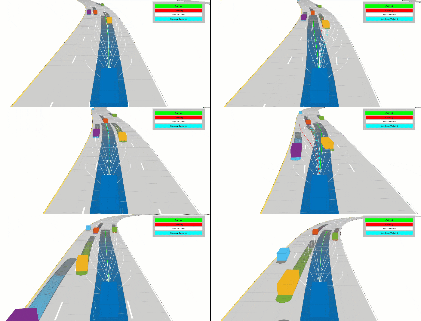
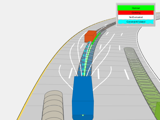
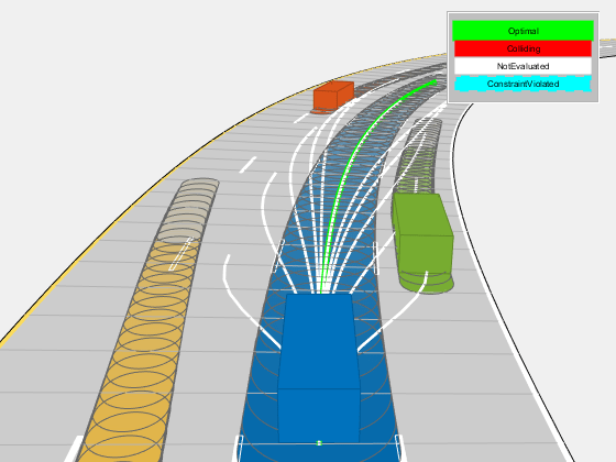
This example uses:

This example demonstrates how to plan a local trajectory in a highway driving scenario. This example uses a reference path and dynamic list of obstacles to generate alternative trajectories for an ego vehicle. The ego vehicle navigates through traffic defined in a provided driving scenario from a drivingScenario object. The vehicle alternates between adaptive cruise control, lane changing, and vehicle following maneuvers based on cost, feasibility, and collision-free motion.

HighwayTrajectoryPlanningUsingFrenetReferencePathExample_01.gif

Load Driving Scenario

Begin by loading the provided drivingScenario object, which defines the vehicle and road properties in the current workspace. This scenario was generated using the Driving Scenario Designer app and exported to a MATLAB® function, drivingScenarioTrafficExample. For more information, see Create Driving Scenario Variations Programmatically.

scenario = drivingScenarioTrafficExample;
% Default car properties
carLen   = 4.7; % in meters
carWidth = 1.8; % in meters
rearAxleRatio = .25;

% Define road dimensions
laneWidth   = carWidth*2; % in meters

plot(scenario);

Figure contains an axes object. The axes object with xlabel X (m), ylabel Y (m) contains 9 objects of type patch, line.

Construct Reference Path

All of the local planning in this example is performed with respect to a reference path, represented by a referencePathFrenet (Navigation Toolbox) object. This object can return the state of the curve at given lengths along the path, find the closest point along the path to some global xy-location, and facilitates the coordinate transformations between global and Frenet reference frames.

For this example, the reference path is treated as the center of a four-lane highway, and the waypoints match the road defined in the provided drivingScenario object.

waypoints = [0 50; 150 50; 300 75; 310 75; 400 0; 300 -50; 290 -50; 0 -50]; % in meters
refPath = referencePathFrenet(waypoints);
ax = show(refPath);
axis(ax,'equal'); xlabel('X'); ylabel('Y');

Figure contains an axes object. The axes object with xlabel X, ylabel Y contains 2 objects of type line. One or more of the lines displays its values using only markers

Construct Trajectory Generator

For a local planner, the goal is typically to sample a variety of possible motions that move towards a final objective while satisfying the current kinematic and dynamic conditions. The trajectoryGeneratorFrenet (Navigation Toolbox) object accomplishes this by connecting the initial state with a set of terminal states using 4th- or 5th-order polynomial trajectories. Initial and terminal states are defined in the Frenet coordinate system, and each polynomial solution satisfies the lateral and longitudinal position, velocity, and acceleration boundary conditions while minimizing jerk.

Terminal states are often calculated using custom behaviors. These behaviors leverage information found in the local environment, such as the lane information, speed limit, and current or future predictions of actors in the ego vehicle's vicinity.

Construct a trajectoryGeneratorFrenet object using the reference path

connector = trajectoryGeneratorFrenet(refPath);

Construct Dynamic Collision Checker

The dynamicCapsuleList (Navigation Toolbox) object is a data structure that represents the state of a dynamic environment over a discrete set of timesteps. This environment can then be used to efficiently validate multiple potential trajectories for the ego vehicle. Each object in the scene is represented by:

Unique integer-valued identifier
Properties for a capsule geometry used for efficient collision checking
Sequence of SE2 states, where each state represents a discrete snapshot in time.

In this example, the trajectories generated by the trajectoryGeneratorFrenet object occur over some span of time, known as the time horizon. To ensure that collision checking covers all possible trajectories, the dynamicCapsuleList object should contain predicted trajectories of all actors spanning the maximum expected time horizon.

capList = dynamicCapsuleList;

Create a geometry structure for the ego vehicle with the given parameters.

egoID = 1;
[egoID, egoGeom] = egoGeometry(capList,egoID);

egoGeom.Geometry.Length = carLen; % in meters
egoGeom.Geometry.Radius = carWidth/2; % in meters
egoGeom.Geometry.FixedTransform(1,end) = -carLen*rearAxleRatio; % in meters

Add the ego vehicle to the dynamic capsule list.

updateEgoGeometry(capList,egoID,egoGeom);

Add the drivingScenario actors to the dynamicCapsuleList object. The geometry is set here, and the states are defined during the planning loop. You can see that the dynamicCapsuleList now contains one ego vehicle and five obstacles.

actorID = (1:5)';
actorGeom = repelem(egoGeom,5,1);
updateObstacleGeometry(capList,actorID,actorGeom)

ans = 
  dynamicCapsuleList with properties:

     MaxNumSteps: 31
          EgoIDs: 1
     ObstacleIDs: [5x1 double]
    NumObstacles: 5
         NumEgos: 1

Planning Adaptive Routes Through Traffic

The planning utilities support a local planning strategy that samples a set of local trajectories based on the current and foreseen state of the environment before choosing the most optimal trajectory. The simulation loop has been organized into the following sections:

Click the titles of each section to navigate to the relevant code in the simulation loop.

Advance Ground Truth Scenario

When planning in a dynamic environment, it is often necessary to estimate the state of the environment or predict its state in the near future. For simplicity, this example uses the drivingScenario as a ground truth source of trajectories for each actor over the planning horizon. To test a custom prediction algorithm, you can replace or modify the exampleHelperRetrieveActorGroundTruth function with custom code.

Generate Terminal States

A common goal in automated driving is to ensure that planned trajectories are not just feasible but also natural. Typical highway driving involves elements of lane keeping, maintaining the speed limit, changing lanes, adapting speed to traffic, and so on. Each custom behavior might require different environment information. This example demonstrates how to generate terminal states that implement three such behaviors: cruise control, lane changes, and follow lead vehicle.

Cruise control

The exampleHelperBasicCruiseControl function generates terminal states that carry out a cruise control behavior. This function uses the ego vehicle's lateral velocity and a time horizon to predict the ego vehicle's expected lane N-seconds in the future. The lane-center is calculated and becomes the terminal state's lateral deviation, and the lateral velocity and acceleration are set to zero.

For longitudinal boundary conditions, the terminal velocity is set to the road speed limit and the terminal acceleration is set to zero. The longitudinal position is unrestricted, which is specified as NaN. By dropping the longitude constraint, trajectoryGeneratorFrenet can use a lower 4th-order polynomial to solve the longitudinal boundary-value problem, resulting in a trajectory that smoothly matches the road speed over the given time horizon:

$c r u i s e C o n t r o l S t a t e = [NaN {\dot{s}}_{d e s} 0 l_{e x p L a n e} 0 0]$

Lane change

The exampleHelperBasicLaneChange function generates terminal states that transition the vehicle from the current lane to either adjacent lane. The function first determines the ego vehicle's current lane, and then checks whether the left and right lanes exist. For each existing lane, the terminal state is defined in the same manner as the cruise control behavior, with the exception that the terminal velocity is set to the current velocity rather than the road's speed limit:

$l a n e C h a n g e S t a t e = [NaN {\dot{s}}_{c u r} 0 l_{d e s L a n e} 0 0]$

Follow lead vehicle

The exampleHelperBasicLeadVehicleFollow function generates terminal states that attempt to trail a vehicle found ahead of the ego vehicle. The function first determines the ego vehicle's current lane. For each provided timeHorizon, the function predicts the future state of each actor, finds all actors that occupy the same lane as the ego vehicle, and determines which is the closest lead vehicle (if no lead vehicles are found, the function does not return anything).

The ego vehicle's terminal state is calculated by taking the lead vehicle's position and velocity and reducing the terminal longitudinal position by some safety distance:

$c l o s e s t L e a d V e h i c l eState = [s_{l e a d} {\dot{s}}_{l e a d} 0 l_{l e a d} {\dot{l}}_{l e a d} 0]$

$followState = [(s_{l e a d} - d_{safety}) {\dot{s}}_{l e a d} 0 l_{l e a d} {\dot{l}}_{l e a d} 0]$

Evaluate Cost of Terminal States

After the terminal states have been generated, their cost can be evaluated. Trajectory evaluation and the ways to prioritize potential solutions is highly subjective. For the sake of simplicity, the exampleHelperEvaluateTSCost function defines cost as the combination of three weighted sums.

Lateral Deviation Cost ( $C_{l a t D e v}$ ) — A positive weight that penalizes states that deviate from the center of a lane.

$C_{l a t D e v} = w_{Δ L} * Δ L$

$Δ L = {argmin}_{i} (| L_{termState} - L_{{lane}_{i}} |)$

Time Cost ( $C_{t i m e}$ ) — A negative weight that prioritizes motions that occur over a longer interval, resulting in smoother trajectories.

$C_{t i m e} = w_{Δ t} * Δ t$

Terminal Velocity Cost ( $C_{s p e e d}$ ) — A positive weight that prioritizes motions that maintain the speed limit, resulting in less dynamic maneuvers.

$C_{s p e e d} = w_{Δ v} * Δ v$

Generate Trajectories and Check for Kinematic Feasibility

In addition to having terminal states with minimal cost, an optimal trajectory must often satisfy additional constraints related to kinematic feasibility and ride comfort. Trajectory constraints are one way of enforcing a desired ride quality, but they do so at the expense of a reduced driving envelope.

In this example, the exampleHelperEvaluateTrajectory function verifies that each trajectory satisfies the following constraints:

MaxAcceleration: The absolute acceleration throughout the trajectory must be below a specified value. Smaller values reduce driving aggressiveness and eliminate kinematically infeasible trajectories. This restriction may eliminate maneuvers that could otherwise be performed by the vehicle.
MaxCurvature: The minimum turning radius that is allowed throughout a trajectory. As with MaxAcceleration, reducing this value results in a smoother driving experience but may eliminate otherwise feasible trajectories.
MinVelocity: This example constrains the ego vehicle to forward-only motion by setting a minimum velocity. This restriction is desired in highway driving scenarios and eliminates trajectories that fit overconstrained or poorly conditioned boundary values.

Check Trajectories for Collision and Select Optimal Trajectory

The final step in the planning process is choosing the best trajectory that also results in a collision-free path. Collision checking is often deferred until the end because it is an expensive operation, so by evaluating cost and analyzing constraints first, invalid trajectories can be removed from consideration. Remaining trajectories can then be checked for collision in optimal order until a collision free path has been found or all trajectories have been evaluated.

Define Simulator and Planning Parameters

This section defines the properties required to run the simulator and parameters that are used by the planner and behavior utilities. Properties such as scenario.SampleTime and connector.TimeResolution are synced so that states in the ground truth actor trajectories and planned ego trajectories occur at the same timesteps. Similarly, replanRate, timeHorizons, and maxHorizon are chosen such that they are integer multiples of the simulation rate.

As mentioned in the previous section, weights and constraints are selected to promote smooth driving trajectories while adhering to the rules of the road.

Lastly, define the speedLimit and safetyGap parameters, which are used to generate terminal states for the planner.

% Synchronize the simulator's update rate to match the trajectory generator's
% discretization interval.
scenario.SampleTime = connector.TimeResolution; % in seconds

% Define planning parameters.
replanRate = 10; % Hz

% Define the time intervals between current and planned states.
timeHorizons = 1:3; % in seconds
maxHorizon = max(timeHorizons); % in seconds

% Define cost parameters.
latDevWeight    =  1;
timeWeight      = -1;
speedWeight     =  1;

% Reject trajectories that violate the following constraints.
maxAcceleration =  15; % in meters/second^2
maxCurvature    =   1; % 1/meters, or radians/meter
minVelocity     =   0; % in meters/second

% Desired velocity setpoint, used by the cruise control behavior and when
% evaluating the cost of trajectories.
speedLimit = 11; % in meters/second

% Minimum distance the planner should target for following behavior.
safetyGap = 10; % in meters

Initialize Simulator

Initialize the simulator and create a chasePlot viewer.

[scenarioViewer,futureTrajectory,actorID,actorPoses,egoID,egoPoses,stepPerUpdate,egoState,isRunning,lineHandles] = ...
    exampleHelperInitializeSimulator(scenario,capList,refPath,laneWidth,replanRate,carLen);

Figure contains an axes object and an object of type uipanel. The hidden axes object with xlabel X (m), ylabel Y (m) contains 9 objects of type patch, line.

Run Driving Simulation

tic
while isRunning
    % Retrieve the current state of actor vehicles and their trajectory over
    % the planning horizon.
    [curActorState,futureTrajectory,isRunning] = ...
        exampleHelperRetrieveActorGroundTruth(scenario,futureTrajectory,replanRate,maxHorizon);

    % Generate cruise control states.
    [termStatesCC,timesCC] = exampleHelperBasicCruiseControl(...
        refPath,laneWidth,egoState,speedLimit,timeHorizons);
    
    % Generate lane change states.
    [termStatesLC,timesLC] = exampleHelperBasicLaneChange(...
        refPath,laneWidth,egoState,timeHorizons);
    
    % Generate vehicle following states.
    [termStatesF,timesF] = exampleHelperBasicLeadVehicleFollow(...
        refPath,laneWidth,safetyGap,egoState,curActorState,timeHorizons);

    % Combine the terminal states and times.
    allTS = [termStatesCC; termStatesLC; termStatesF];
    allDT = [timesCC; timesLC; timesF];
    numTS = [numel(timesCC); numel(timesLC); numel(timesF)];
    
    % Evaluate cost of all terminal states.
    costTS = exampleHelperEvaluateTSCost(allTS,allDT,laneWidth,speedLimit,...
        speedWeight, latDevWeight, timeWeight);

    % Generate trajectories.
    egoFrenetState = global2frenet(refPath,egoState);
    [frenetTraj,globalTraj] = connect(connector,egoFrenetState,allTS,allDT);
    
    % Eliminate trajectories that violate constraints.
    isValid = exampleHelperEvaluateTrajectory(globalTraj,maxAcceleration,maxCurvature,minVelocity);

    % Update the collision checker with the predicted trajectories
    % of all actors in the scene.
    for i = 1:numel(actorPoses)
        actorPoses(i).States = futureTrajectory(i).Trajectory(:,1:3);
    end
    updateObstaclePose(capList,actorID,actorPoses);
    
    % Determine evaluation order.
    [cost, idx] = sort(costTS);
    optimalTrajectory = [];
    
    trajectoryEvaluation = nan(numel(isValid),1);
    
    % Check each trajectory for collisions starting with least cost.
    for i = 1:numel(idx)
        if isValid(idx(i))
            % Update capsule list with the ego object's candidate trajectory.
            egoPoses.States = globalTraj(idx(i)).Trajectory(:,1:3);
            updateEgoPose(capList,egoID,egoPoses);
            
            % Check for collisions.
            isColliding = checkCollision(capList);
            
            if all(~isColliding)
                % If no collisions are found, this is the optimal.
                % trajectory.
                trajectoryEvaluation(idx(i)) = 1;
                optimalTrajectory = globalTraj(idx(i)).Trajectory;
                break;
            else
                trajectoryEvaluation(idx(i)) = 0;
            end
        end
    end

    % Display the sampled trajectories.
    lineHandles = exampleHelperVisualizeScene(lineHandles,globalTraj,isValid,trajectoryEvaluation);
    
    hold on;
    show(capList,'TimeStep',1:capList.MaxNumSteps,'FastUpdate',1);
    hold off;
    
    if isempty(optimalTrajectory)
        % All trajectories either violated a constraint or resulted in collision.
        %
        %   If planning failed immediately, revisit the simulator, planner,
        %   and behavior properties.
        %
        %   If the planner failed midway through a simulation, additional
        %   behaviors can be introduced to handle more complicated planning conditions.
        error('No valid trajectory has been found.');
    else
        % Visualize the scene between replanning.
        for i = (2+(0:(stepPerUpdate-1)))
            % Approximate realtime visualization.
            dt = toc;
            if scenario.SampleTime-dt > 0
                pause(scenario.SampleTime-dt);
            end
            
            egoState = optimalTrajectory(i,:);
            scenarioViewer.Actors(1).Position(1:2) = egoState(1:2);
            scenarioViewer.Actors(1).Velocity(1:2) = [cos(egoState(3)) sin(egoState(3))]*egoState(5);
            scenarioViewer.Actors(1).Yaw = egoState(3)*180/pi;
            scenarioViewer.Actors(1).AngularVelocity(3) = egoState(4)*egoState(5);
            
            % Update capsule visualization.
            hold on;
            show(capList,'TimeStep',i:capList.MaxNumSteps,'FastUpdate',1);
            hold off;
            
            % Update driving scenario.
            advance(scenarioViewer);
            tic;
        end
    end
end

Figure contains an axes object and an object of type uipanel. The hidden axes object with xlabel X (m), ylabel Y (m) contains 35 objects of type patch, line.

Planner Customizations and Additional Considerations

Custom solutions often involve many tunable parameters, each capable of changing the final behavior in ways that are difficult to predict. This section highlights some of the feature-specific properties and their effect on the above planner. Then, suggestions provide ways to tune or augment the custom logic.

Dynamic Capsule List

As mentioned previously, the dynamicCapsuleList object acts as a temporal database, which caches predicted trajectories of obstacles. You can perform collision checking with one or more ego bodies over some span of time. The MaxNumSteps property determines the total number of time-steps that are checked by the object. In the above simulation loop, the property was set to 31. This value means the planner checks the entire 1-3 second span of any trajectories (sampled at every 0.1 second). Now, increase the maximum value in timeHorizons:

timeHorizons   = 1:5; % in seconds
maxTimeHorizon = max(timeHorizons); % in seconds

There are now two options:

The MaxNumSteps property is left unchanged.
The MaxNumSteps property is updated to accommodate the new max timespan.

If the property is left unchanged, then the capsule list only validates the first 3 seconds of any trajectory, which may be preferable if computational efficiency is paramount or the prediction certainty drops off quickly.

Alternatively, one may be working with ground truth data (as is shown above), or the future state of the environment is well known (e.g. a fully automated environment with centralized control). Since this example uses ground truth data for the actors, update the property.

capList.MaxNumSteps = 1+floor(maxTimeHorizon/scenario.SampleTime);

Another, indirectly tunable, property of the list is the capsule geometry. The geometry of the ego vehicle or actors can be inflated by increasing the Radius, and buffer regions can be added to vehicles by modifying the Length and FixedTransform properties.

Inflate the ego vehicle's entire footprint by increasing the radius.

egoGeom.Geometry.Radius = laneWidth/2; % in meters
updateEgoGeometry(capList,egoID,egoGeom);

Add a front and rear buffer region to all actors.

actorGeom(1).Geometry.Length = carLen*1.5; % in meters
actorGeom(1).Geometry.FixedTransform(1,end) = -actorGeom(1).Geometry.Length*rearAxleRatio; % in meters
actorGeom = repmat(actorGeom(1),5,1);
updateObstacleGeometry(capList,actorID,actorGeom);

Rerun Simulation With Updated Properties

Rerun the simulation. The resulting simulation has a few interesting developments:

The longer five-second time horizon results in a much smoother driving experience. The planner still prioritizes the longer trajectories due to the negative timeWeight.
The updated MaxNumSteps property has enabled collision checking over the full trajectory. When paired with the longer planning horizon, the planner identifies and discards the previously optimal left-lane change and returns to the original lane.
The inflated capsules find a collision earlier and reject a trajectory, which results in more conservative driving behavior. One potential drawback to this is a reduced planning envelope, which runs the risk of the planner not being able to find a valid trajectory.

% Initialize the simulator and create a chasePlot viewer.
[scenarioViewer,futureTrajectory,actorID,actorPoses,egoID,egoPoses,stepPerUpdate,egoState,isRunning,lineHandles] = ...
    exampleHelperInitializeSimulator(scenario,capList,refPath,laneWidth,replanRate,carLen);
tic;
while isRunning
    % Retrieve the current state of actor vehicles and their trajectory over
    % the planning horizon.
    [curActorState,futureTrajectory,isRunning] = exampleHelperRetrieveActorGroundTruth(...
        scenario,futureTrajectory,replanRate,maxHorizon);
    
    % Generate cruise control states.
    [termStatesCC,timesCC] = exampleHelperBasicCruiseControl(...
        refPath,laneWidth,egoState,speedLimit,timeHorizons);
    
    % Generate lane change states.
    [termStatesLC,timesLC] = exampleHelperBasicLaneChange(...
        refPath,laneWidth,egoState,timeHorizons);
    
    % Generate vehicle following states.
    [termStatesF,timesF] = exampleHelperBasicLeadVehicleFollow(...
        refPath,laneWidth,safetyGap,egoState,curActorState,timeHorizons);
    
    % Combine the terminal states and times.
    allTS = [termStatesCC; termStatesLC; termStatesF];
    allDT = [timesCC; timesLC; timesF];
    numTS = [numel(timesCC); numel(timesLC); numel(timesF)];
    
    % Evaluate cost of all terminal states.
    costTS = exampleHelperEvaluateTSCost(allTS,allDT,laneWidth,speedLimit, ...
        speedWeight,latDevWeight,timeWeight);
    
    % Generate trajectories.
    egoFrenetState = global2frenet(refPath,egoState);
    [frenetTraj,globalTraj] = connect(connector,egoFrenetState,allTS,allDT);
    
    % Eliminate trajectories that violate constraints.
    isValid = exampleHelperEvaluateTrajectory(...
        globalTraj, maxAcceleration, maxCurvature, minVelocity);
    
    % Update the collision checker with the predicted trajectories
    % of all actors in the scene.
    for i = 1:numel(actorPoses)
        actorPoses(i).States = futureTrajectory(i).Trajectory(:,1:3);
    end
    updateObstaclePose(capList, actorID, actorPoses);
    
    % Determine evaluation order.
    [cost, idx] = sort(costTS);
    optimalTrajectory = [];
    
    trajectoryEvaluation = nan(numel(isValid),1);
    
    % Check each trajectory for collisions starting with least cost.
    for i = 1:numel(idx)
        if isValid(idx(i))
            % Update capsule list with the ego object's candidate trajectory.
            egoPoses.States = globalTraj(idx(i)).Trajectory(:,1:3);
            updateEgoPose(capList, egoID, egoPoses);
            
            % Check for collisions.
            isColliding = checkCollision(capList);
            
            if all(~isColliding)
                % If no collisions are found, this is the optimal
                % trajectory.
                trajectoryEvaluation(idx(i)) = 1;
                optimalTrajectory = globalTraj(idx(i)).Trajectory;
                break;
            else
                trajectoryEvaluation(idx(i)) = 0;
            end
        end
    end
    
    % Display the sampled trajectories.
    lineHandles = exampleHelperVisualizeScene(lineHandles, globalTraj, isValid, trajectoryEvaluation);
    
    if isempty(optimalTrajectory)
        % All trajectories either violated a constraint or resulted in collision.
        %
        %   If planning failed immediately, revisit the simulator, planner,
        %   and behavior properties.
        %
        %   If the planner failed midway through a simulation, additional
        %   behaviors can be introduced to handle more complicated planning conditions.
        error('No valid trajectory has been found.');
    else
        % Visualize the scene between replanning.
        for i = (2+(0:(stepPerUpdate-1)))
            % Approximate realtime visualization.
            dt = toc;
            if scenario.SampleTime-dt > 0
                pause(scenario.SampleTime-dt);
            end
            
            egoState = optimalTrajectory(i,:);
            scenarioViewer.Actors(1).Position(1:2) = egoState(1:2);
            scenarioViewer.Actors(1).Velocity(1:2) = [cos(egoState(3)) sin(egoState(3))]*egoState(5);
            scenarioViewer.Actors(1).Yaw = egoState(3)*180/pi;
            scenarioViewer.Actors(1).AngularVelocity(3) = egoState(4)*egoState(5);
            
            % Update capsule visualization.
            hold on;
            show(capList,'TimeStep',i:capList.MaxNumSteps,'FastUpdate',1);
            hold off;
            
            % Update driving scenario.
            advance(scenarioViewer);
            tic;
        end
    end
end