PIL Verification of Generated Code for Map Creation Using Lidar SLAM

This example uses:

This example shows how to design, simulate, and generate embedded code for building a map from lidar data using the simultaneous localization and mapping (SLAM) algorithm, and verify it using processor-in-the-loop (PIL) simulation on NVIDIA® Jetson™ hardware. In this example, you:

Design and simulate map creation from lidar data using normal-distributions transform (NDT) and lidar odometry and mapping (LOAM) algorithms in Simulink® and compare their performance.
Configure the model to run a PIL simulation and verify the results against normal simulation.

Introduction

SLAM is a process of calculating the position and orientation of a vehicle, with respect to its surroundings, while simultaneously building a map of the environment around the vehicle. This example uses 3D point cloud data from a lidar sensor and measurements from an inertial navigation system (INS) sensor to progressively build a map and estimate the trajectory of the ego vehicle. You can also test the SLAM algorithm for map creation on NVIDIA Jetson hardware using PIL simulation. A PIL simulation runs the generated code on your target hardware. You can verify the numerical equivalence between your model and the generated code by comparing the results of normal and PIL simulations.

In this example, you:

Explore Test Bench Model — The model contains sensors and an environment, a map creation algorithm using point cloud registration, and metrics to assess functionality.
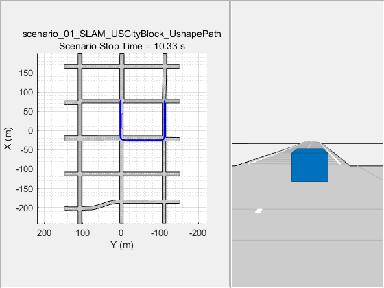
Visualize Test Scenario — The scenario contains a U-shaped trajectory in US City Block scene.
Simulate Model — Configure the test bench model for a test scenario containing a U-shaped trajectory. Simulate the model using NDT and LOAM variants and compare their results.
Generate C++ Code — Configure the reference model to generate C++ code.
Run PIL Simulation — Perform PIL simulation on NVIDIA Jetson hardware, and assess the results.
Explore Other Scenarios — Simulate the model for other scenarios, and assess the results.

This example tests map creation, from lidar data using a SLAM algorithm, in a 3D simulation environment that uses the Unreal Engine® from Epic Games®.

if ~ispc
    error(['This example is supported only on Microsoft', char(174), ...
        ' Windows', char(174), '.'])
end

To ensure reproducibility of the simulation results, set the random number generator seed.

rng(0)

Explore Test Bench Model

Open the test bench model.

open_system("LidarSLAMMapCreationTestBench")

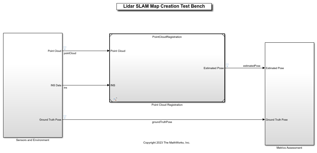
Opening this model runs the helperSLLidarSLAMMapCreationSetup helper function, which initializes the scenario using a drivingScenario object in the base workspace. It also configures the sensors required for defining the inputs and outputs for the LidarSLAMMapCreationTestBench model. The test bench model contains these subsystems:

Sensors and Environment — Specifies the scene and sensors used for simulation.
Point Cloud Registration — Aligns successive lidar scans by using NDT or LOAM algorithm. For more information on NDT and LOAM algorithms, see pcregisterndt and pcregisterloam (Lidar Toolbox), respectively.
Metrics Assessment — Assesses the point cloud registration performance using the root-mean-square error (RMSE) metric between the estimated pose and ground truth pose of the ego vehicle.

Configure Sensors and Environment

The Sensors and Environment subsystem configures the road network, sets the vehicle positions, and synthesizes the sensors. Open the Sensors and Environment subsystem.

open_system("LidarSLAMMapCreationTestBench/Sensors and Environment")

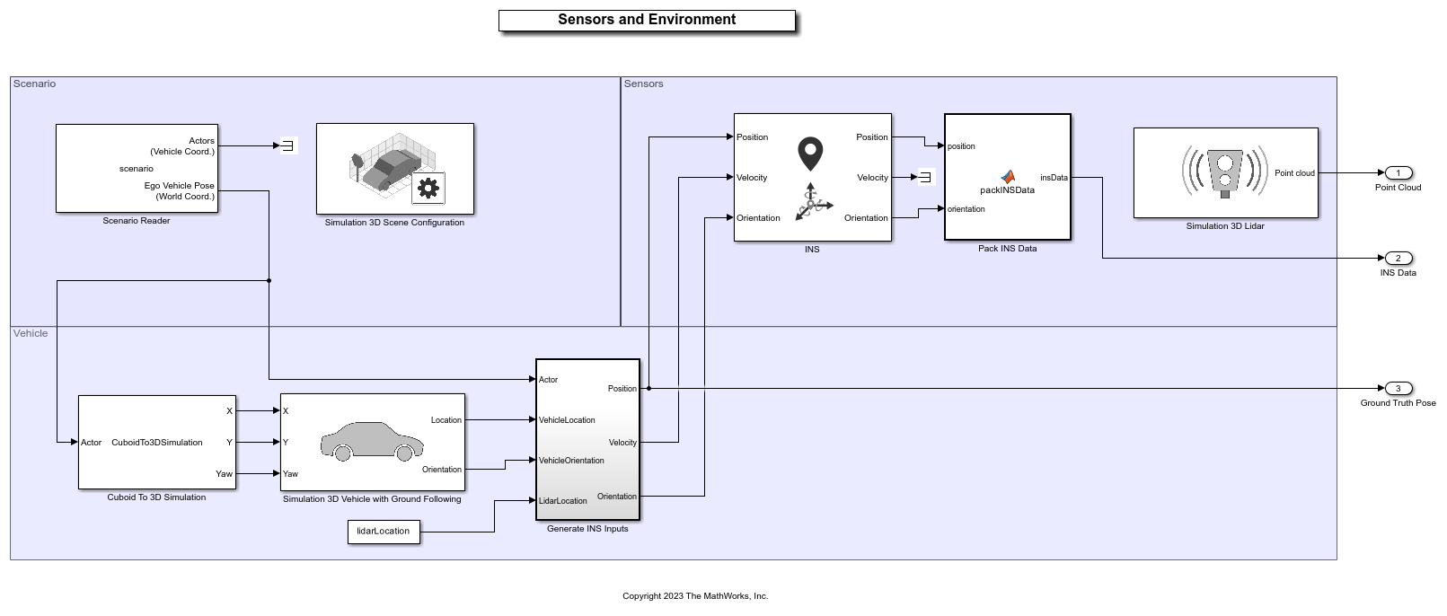
These parts of the subsystem specify the scene and road network:

The Simulation 3D Scene Configuration block has the SceneName parameter set to US city block.
The Scenario Reader block has been configured to use a driving scenario that contains a road network that closely matches the road network from the US City Block scene.

The example specifies vehicle positions by using these parts of the subsystem:

The Scenario Reader block outputs the pose of the ego vehicle specified by the Simulation 3D Vehicle with Ground Following block.
The Cuboid To 3D Simulation block converts the ego pose coordinate system, with an origin below the center of the vehicle rear axle, to the 3D simulation coordinate system, with an origin below the vehicle center.
The Generate INS Inputs block computes the position, velocity, and orientation of the ego vehicle with reference to the sensor placement using the pose information received from the Scenario Reader block and Simulation 3D Vehicle with Ground Following block. This information is useful for providing inputs to the INS sensor block and computing the ground truth pose.
The INS (Navigation Toolbox) block models the measurements from the inertial navigation system, and global navigation satellite system and outputs the fused measurements. It outputs the noise-corrupted position, velocity, and orientation for the ego vehicle.
The Pack INS Data block packs INS block output into the format required by the NDT and LOAM algorithms for point cloud registration.
The constant block gives lidar sensor location relative to vehicle origin mounted at roof center.
The Simulation 3D Lidar block models a lidar sensor in a 3D simulation environment, and generates detections in the form of point cloud data. This sensor is mounted to the center of the roof of the ego vehicle.

Perform Point Cloud Registration

To build a map from lidar data, this example uses the Point Cloud Registration reference model. Open the model.

open_system("PointCloudRegistration")

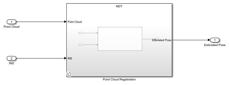
The Point Cloud Registration reference model contains a variant subsystem. It contains two variants for point cloud registration. You can configure the desired variant using the helperSLLidarSLAMMapCreationSetup function.

NDT — This is the default variant. This variant aligns successive lidar scans by using the pcregisterndt function, which registers two point clouds using the NDT algorithm. By successively composing these transformations, the variant transforms each point cloud back to the reference frame of the first point cloud. Consequently, the variant generates a map by combining all the transformed point clouds.

Open the NDT variant.

open_system("PointCloudRegistration/Point Cloud Registration/NDT")

LOAM — This variant uses the pcregisterloam function to register point clouds using the LOAM algorithm. The algorithm extracts features such as edge points and surface points from lidar scans to build a map.

Configure the LOAM variant using the helperSLLidarSLAMMapCreationSetup function.

helperSLLidarSLAMMapCreationSetup("registrationVariantName","LOAM")

Open the LOAM variant.

open_system("PointCloudRegistration/Point Cloud Registration/LOAM")

Evaluate Performance of Point Cloud Registration

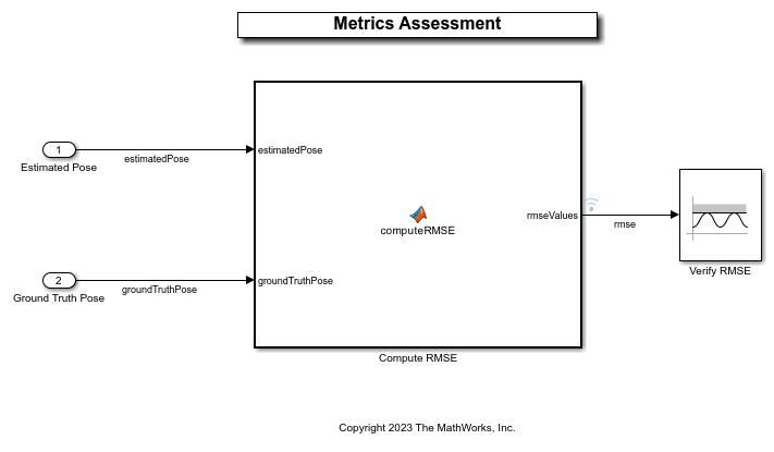
The Metrics Assessment subsystem computes the RMSE between the ground truth pose and the estimated pose from the point cloud registration algorithm.

open_system("LidarSLAMMapCreationTestBench/Metrics Assessment")

Visualize Test Scenario

The helperPlotScenario helper function generates a cuboid scenario that is compatible with the LidarSLAMMapCreationTestBench model.

Plot the open-loop scenario, and visualize the ego path.

hFigScenario = helperPlotScenario("scenario_01_SLAM_USCityBlock_UshapePath");

Close the figure.

close(hFigScenario)

Simulate Model

In this section, you simulate the model with the NDT and LOAM registration algorithms, and compare their results using a test scenario.

Simulate Model Using NDT Algorithm

Configure the LidarSLAMMapCreationTestBench model to use the scenario_01_SLAM_USCityBlock_UshapePath scenario and NDT registration variant. In this scenario, the ego vehicle travels a U-shaped path in a US City Block scenario.

helperSLLidarSLAMMapCreationSetup("registrationVariantName","NDT","scenarioFcnName","scenario_01_SLAM_USCityBlock_UshapePath")

Simulate the test bench model.

simoutNDT = sim("LidarSLAMMapCreationTestBench");

While running the simulation, the model generates the RMSE metric. The model logs metric, along with the estimated pose, ground truth pose, and point cloud locations information, to the base workspace variable simoutNDT.logsout.

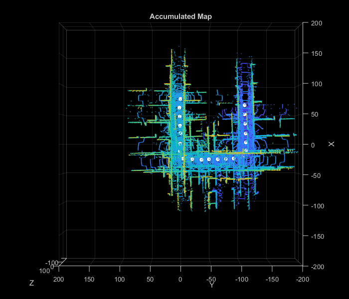
Visualize the accumulated map by using the helperLidarSLAMMapCreationAndVisualization helper function.

hPCPlayer = helperLidarSLAMMapCreationAndVisualization(simoutNDT.logsout);

Hide the point cloud player.

hide(hPCPlayer)

Simulate Model Using LOAM Algorithm

Configure the LidarSLAMMapCreationTestBench model to use the scenario_01_SLAM_USCityBlock_UshapePath scenario and LOAM registration variant. In this scenario, the ego vehicle travels a U-shaped path in a US City Block scenario.

helperSLLidarSLAMMapCreationSetup("registrationVariantName","LOAM","scenarioFcnName","scenario_01_SLAM_USCityBlock_UshapePath")

Simulate the test bench model.

simoutLOAM = sim("LidarSLAMMapCreationTestBench");

While running the simulation, the model logs RMSE metric, along with the estimated pose, ground truth pose, and point cloud locations information, to the base workspace variable simoutLOAM.logsout.

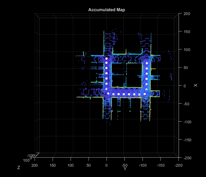
Visualize the accumulated map by using the helperLidarSLAMMapCreationAndVisualization helper function.

hPCPlayer = helperLidarSLAMMapCreationAndVisualization(simoutLOAM.logsout);

Hide the point cloud player.

hide(hPCPlayer)

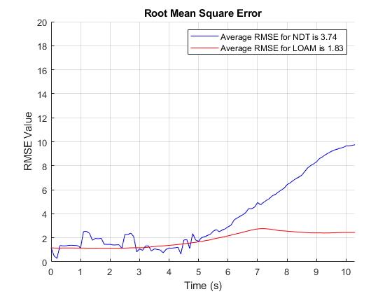
Compare the overall performance of the NDT and LOAM registration algorithms by plotting the RMSE values.

hFigCompareResults = helperPlotRMSEComaparisonResults(simoutNDT.logsout,simoutLOAM.logsout);

Close the figure.

close(hFigCompareResults)

The plot indicates that LOAM performs better than NDT for this test scenario.

Generate C++ Code

You can now generate C++ code for the NDT or LOAM algorithm, apply common optimizations, and generate a report to facilitate exploring the generated code. This example configures the model to use the NDT algorithm.

helperSLLidarSLAMMapCreationSetup("registrationVariantName","NDT")

Configure the Point Cloud Registration model to generate C++ code for real-time implementation of the algorithm. Set the model parameters to enable code generation, and display the configuration values.

Generate code for the reference model.

slbuild("PointCloudRegistration")

Run PIL Simulation

After generating the C++ code, you can now verify the code using PIL simulation on an NVIDIA Jetson board. The PIL simulation enables you to test the functional equivalence of the compiled, generated code on the intended hardware. For more information about PIL simulation, see SIL and PIL Simulations (Embedded Coder).

Follow these steps to perform a PIL simulation.

1. Create a hardware object for an NVIDIA Jetson board.

hwObj = jetson("jetson-name","ubuntu","ubuntu");

2. Set up the model configuration parameters for the Point Cloud Registration reference model.

% Set the hardware board.
load_system("PointCloudRegistration")
set_param("PointCloudRegistration",HardwareBoard="NVIDIA Jetson")
save_system("PointCloudRegistration")

% Set model parameters for PIL simulation.
set_param("LidarSLAMMapCreationTestBench/Point Cloud Registration",SimulationMode="Processor-in-the-loop")

3. Simulate the model, and observe the behavior.

pilSimOut = sim("LidarSLAMMapCreationTestBench");

Compare the outputs from normal simulation mode and PIL simulation mode.

runIDs = Simulink.sdi.getAllRunIDs;
normalSimRunID = runIDs(end - 2);
pilSimRunID = runIDs(end);
normalSimRun = Simulink.sdi.getRun(normalSimRunID);
pilSimRun = Simulink.sdi.getRun(pilSimRunID);
normalSimRunRMSEsig = getSignalIDByIndex(normalSimRun,1);
pilSimRunRMSESig = getSignalIDByIndex(pilSimRun,1);

diffResult = Simulink.sdi.compareSignals(normalSimRunRMSEsig,pilSimRunRMSESig);

Plot the differences in the RMSE metrics computed from normal mode and PIL mode.

hFigDiffResults = helperPlotRMSEDiffResults(diffResult);

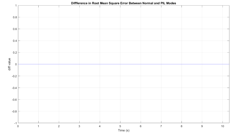
Note that the RMSE metrics captured during both runs are the same, indicating that the PIL mode simulation produces the same results as the normal mode simulation.

Close the figure.

close(hFigDiffResults)

Assess Execution Time

During the PIL simulation, the host computer logs the execution-time metrics for the deployed code to the pilSimOut.executionProfile variable in the MATLAB® base workspace. You can use the execution-time metrics to determine whether the generated code meets the requirements for real-time deployment on your target hardware. These times indicate the performance of the generated code on the target hardware. For more information, see Create Execution-Time Profile for Generated Code (Embedded Coder).

Plot the execution time for the PointCloudRegistration_step function.

helperPlotExecutionProfile(pilSimOut.executionProfile)

Using the plot, you can deduce the average time that the Point Cloud Registration model takes to execute each frame. For more information on generating execution profiles and analyzing them during SIL simulation, see Execution Time Profiling for SIL and PIL (Embedded Coder).

Explore Other Scenarios

You can use the procedure in this example to explore these other scenarios, which are compatible with the LidarSLAMMapCreationTestBench model:

scenario_01_SLAM_USCityBlock_UshapePath (default)
scenario_02_SLAM_USCityBlock_EightshapePath
scenario_03_SLAM_USCityBlock_LshapePath

Use these additional scenarios to analyze the LidarSLAMMapCreationTestBench model results for different paths.

PIL Verification of Generated Code for Map Creation Using Lidar SLAM

Introduction

Explore Test Bench Model

Visualize Test Scenario

Simulate Model

Generate C++ Code

Run PIL Simulation

Explore Other Scenarios

See Also

Blocks

Functions

Related Topics