designHalfbandFIR
Description
B = designHalfbandFIRB is a vector of halfband FIR coefficients of length 25.
The System object™ argument is false by default. To implement the filter,
assign the filter coefficients in B to one of the supported System
objects.
B = designHalfbandFIR(Name=Value)
For example, B =
designHalfbandFIR(FilterOrder=30,TransitionWidth=0.2,DesignMethod="kaiser",SystemObject=true)SystemObject argument
is true, the function designs and implements the halfband FIR filter.
B is a dsp.FIRFilter
System object in this case.
When you specify only a partial list of filter parameters, the function designs the filter by setting the other design parameters to their default values.
When you specify any of the numeric input arguments in single precision, the function
designs the filter coefficients in single precision. Alternatively, you can use the Datatype and
like arguments to control the data type of the
coefficients. (since R2024b)
The function supports three design methods. Each design method supports a specific
set of design combinations. For more information, see DesignMethod.
This function supports code generation under certain conditions. For more information, see Code Generation.
Examples
Since R2024b
Use the designHalfbandFIR function to design a minimum-phase FIR halfband filter. Set PhaseConstraint to "minimum" and InputSampleRate to 1200 Hz.
minHalfband = designHalfbandFIR(FilterOrder=49,...
    PhaseConstraint='minimum',InputSampleRate=1200,...
    SystemObject=true,Verbose=true)
designHalfbandFIR(FilterOrder=49, TransitionWidth=60, DesignMethod="equiripple", Passband="lowpass", Structure="single-rate", InputSampleRate=1200, PhaseConstraint="minimum", Datatype="double", SystemObject=true)
minHalfband =
  dsp.FIRFilter with properties:

            Structure: 'Direct form'
      NumeratorSource: 'Property'
            Numerator: [0.0880 0.2902 0.4470 0.3323 4.6647e-04 -0.1975 -0.0760 0.1161 0.0842 -0.0719 -0.0773 0.0471 0.0676 -0.0327 -0.0580 0.0239 0.0494 -0.0184 -0.0419 0.0149 0.0354 -0.0125 -0.0297 0.0109 0.0247 -0.0097 -0.0203 0.0086 … ] (1×50 double)
    InitialConditions: 0

  Show all properties
Visualize the magnitude response of this filter using filterAnalyzer.
filterAnalyzer(minHalfband)
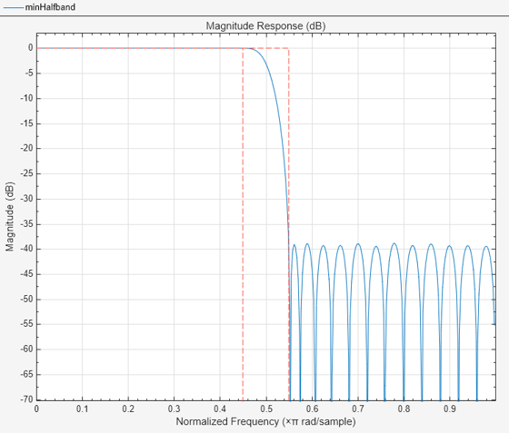
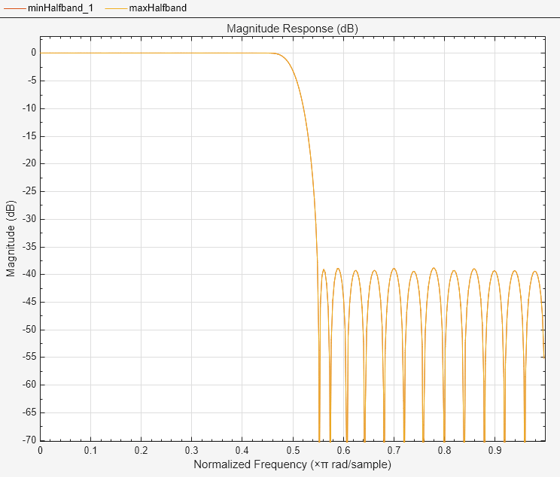
Set PhaseConstraint to 'maximum' to design a maximum-phase FIR halfband filter. With the same specifications, notice that the magnitude response of the minimum-phase and maximum-phase filters is identical.
maxHalfband = designHalfbandFIR(FilterOrder=49,...
    PhaseConstraint='maximum',InputSampleRate=1200,...
    SystemObject=true,Verbose=true)
designHalfbandFIR(FilterOrder=49, TransitionWidth=60, DesignMethod="equiripple", Passband="lowpass", Structure="single-rate", InputSampleRate=1200, PhaseConstraint="maximum", Datatype="double", SystemObject=true)
maxHalfband =
  dsp.FIRFilter with properties:

            Structure: 'Direct form'
      NumeratorSource: 'Property'
            Numerator: [7.4348e-04 -0.0024 0.0031 -6.5203e-04 -0.0024 0.0012 0.0027 -0.0019 -0.0033 0.0029 0.0040 -0.0041 -0.0047 0.0058 0.0055 -0.0079 -0.0062 0.0103 0.0070 -0.0132 -0.0078 0.0165 0.0086 -0.0203 -0.0097 0.0247 0.0109 … ] (1×50 double)
    InitialConditions: 0

  Show all properties
filterAnalyzer(minHalfband,maxHalfband)
Compare the phase response of the two filters.
filterAnalyzer(minHalfband,maxHalfband,Analysis="phase")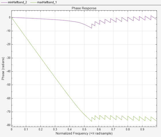
Compare the impulse response of the two filters. For the minimum-phase FIR filter, the energy of its impulse response is maximally concentrated towards the beginning of the impulse response, while the opposite is true for the maximum-phase filter.
filterAnalyzer(minHalfband,maxHalfband,Analysis="impulse")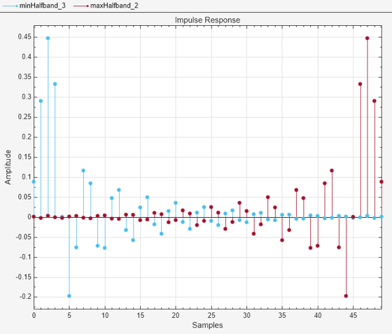
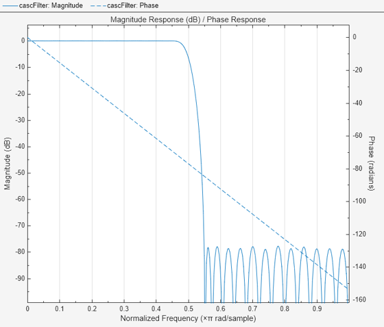
Cascading the minimum- and maximum-phase filters yields a linear phase filter. The magnitude response of the filter cascade is the same as the individual filters but the phase response is linear.
cascFilter = cascade(minHalfband,maxHalfband)
cascFilter =
  dsp.FilterCascade with properties:

         Stage1: [1×1 dsp.FIRFilter]
         Stage2: [1×1 dsp.FIRFilter]
    CloneStages: true
filterAnalyzer(cascFilter,Analysis="magnitude",OverlayAnalysis="phase")
Design an equiripple FIR halfband filter with the order of 24 and a transition width of 0.1 using the designHalfbandFIR function. Assign the filter coefficients to a dsp.FIRFilter System object.
b = designHalfbandFIR(FilterOrder=24,DesignMethod="equiripple");
hbFIR = dsp.FIRFilter(b);
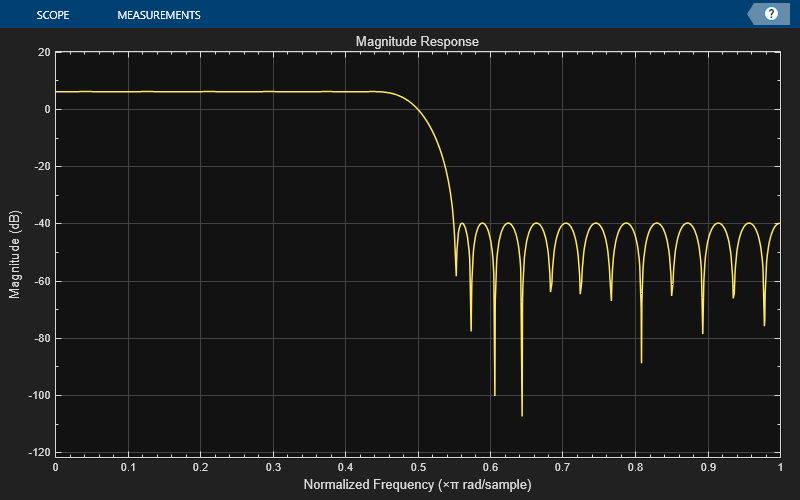
Create a dsp.DynamicFilterVisualizer object and visualize the magnitude response of the filter.
dfv = dsp.DynamicFilterVisualizer(NormalizedFrequency=true);
dfv(hbFIR);

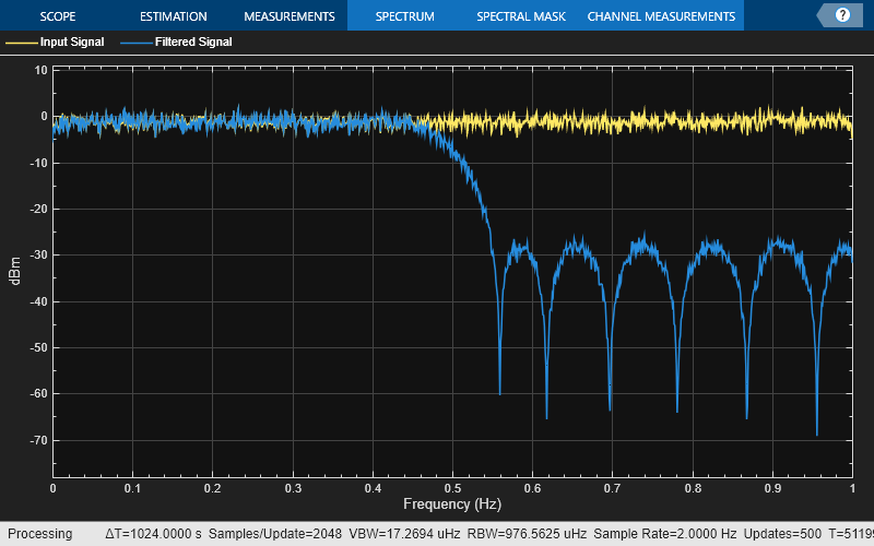
Create a spectrumAnalyzer object to visualize the spectra of the input and output signals.
scope = spectrumAnalyzer(SampleRate=2, PlotAsTwoSidedSpectrum=false,...
    ChannelNames=["Input Signal","Filtered Signal"]);
Stream in random data and filter the signal using the FIR halfband filter.
for i = 1:1000
    x = randn(1024, 1);
    y = hbFIR(x);
    scope(x,y);
end
Design an equiripple FIR halfband interpolator object of order 48 using the designHalfbandFIR function. Set the Verbose argument to true.
hbFIR = designHalfbandFIR(FilterOrder=48,SystemObject=true,...
    Structure="interp",Verbose=true)
designHalfbandFIR(FilterOrder=48, TransitionWidth=0.1, DesignMethod="equiripple", Passband="lowpass", Structure="interp", InputSampleRate="normalized", PhaseConstraint="linear", Datatype="double", SystemObject=true)
hbFIR =
  dsp.FIRHalfbandInterpolator with properties:

          Specification: 'Coefficients'
              Numerator: [0 -0.0082 0 0.0079 0 -0.0116 0 0.0165 0 -0.0227 0 0.0309 0 -0.0419 0 0.0571 0 -0.0800 0 0.1193 0 -0.2073 0 0.6350 1 0.6350 0 -0.2073 0 0.1193 0 -0.0800 0 0.0571 0 -0.0419 0 0.0309 0 -0.0227 0 0.0165 0 -0.0116 0 … ] (1×49 double)
    FilterBankInputPort: false

  Show all properties
Create a dsp.DynamicFilterVisualizer object and visualize the magnitude response of the filter.
dfv = dsp.DynamicFilterVisualizer(NormalizedFrequency=true);
dfv(hbFIR);
The input is a cosine wave with an angular frequency of radians/sample.
input = cos(pi/4*(0:39)');
Interpolate the cosine signal using the FIR halfband interpolator.
output = hbFIR(input);
Plot the original and interpolated signals. In order to plot the two signals on the same plot, you must account for the output delay introduced by the FIR halfband interpolator and the scaling introduced by the filter. Use the outputDelay function to compute the delay value introduced by the interpolator. Shift the output by this delay value.
Visualize the input and the resampled signals. The input and output values coincide every other sample due to the interpolation factor of 2.
[delay,FsOut] = outputDelay(hbFIR,FsIn=1)
delay =
12
FsOut =
2
nInput = (0:length(input)-1);
tOutput = (0:length(output)-1)/FsOut-delay;
stem(tOutput,output,"filled",MarkerSize=4); hold on;
stem(nInput,input); hold off;
xlim([-5,20])
legend("Interpolated by 2","Input signal",Location="best");

Design an equiripple FIR halfband decimator object of order 48 using the designHalfbandFIR function. Set the Verbose argument to true.
hbFIR = designHalfbandFIR(FilterOrder=48,SystemObject=true,...
    Structure="decim",Verbose=true)
designHalfbandFIR(FilterOrder=48, TransitionWidth=0.1, DesignMethod="equiripple", Passband="lowpass", Structure="decim", InputSampleRate="normalized", PhaseConstraint="linear", Datatype="double", SystemObject=true)
hbFIR =
  dsp.FIRHalfbandDecimator with properties:

   Main
    Specification: 'Coefficients'
        Numerator: [0 -0.0041 0 0.0040 0 -0.0058 0 0.0082 0 -0.0114 0 0.0155 0 -0.0209 0 0.0286 0 -0.0400 0 0.0597 0 -0.1037 0 0.3175 0.5000 0.3175 0 -0.1037 0 0.0597 0 -0.0400 0 0.0286 0 -0.0209 0 0.0155 0 -0.0114 0 0.0082 0 -0.0058 0 0.0040 0 -0.0041 0]

  Show all properties
Create a dsp.DynamicFilterVisualizer object and visualize the magnitude response of the filter.
dfv = dsp.DynamicFilterVisualizer(NormalizedFrequency=true);
dfv(hbFIR);

The input is a cosine wave with an angular frequency of radians/sample.
input = cos(pi/4*(0:39)');
Decimate the cosine signal using the FIR halfband decimator.
output = hbFIR(input);
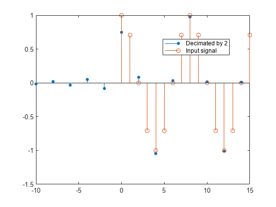
Plot the original and decimated signals. In order to plot the two signals in the same plot, you must account for the output delay of the FIR halfband decimator and the scaling introduced by the filter. Use the outputDelay function to compute the delay introduced by the decimator. Shift the output by this delay value.
Visualize the input and the resampled signals. After a short transition, the output converges to a cosine of frequency , as expected, which is twice the frequency of the input signal, . Due to the decimation factor of 2, the output samples coincide with every other input sample.
[delay,FsOut] = outputDelay(hbFIR,FsIn=1)
delay =
24
FsOut =
0.5000
nInput = (0:length(input)-1);
tOutput = (0:length(output)-1)/FsOut-delay;
stem(tOutput,output,"filled",MarkerSize=4); hold on;
stem(nInput,input); hold off;
xlim([-10,15])
legend("Decimated by 2","Input signal","Location","best");
Name-Value Arguments
Specify optional pairs of arguments as
Name1=Value1,...,NameN=ValueN, where Name is
the argument name and Value is the corresponding value.
Name-value arguments must appear after other arguments, but the order of the
pairs does not matter.
Example:
designHalfbandFIR(FilterOrder=30,TransitionWidth=0.3,Passband="lowpass")
Order of the halfband FIR filter, N, specified as one of these:
Positive even integer when you set
PhaseConstraintto"linear"(linear-phase Kaiser design).Positive odd integer when you set
PhaseConstraintto"minimum"(minimum-phase design) or"maximum"(maximum-phase design).
This property is tunable in code
generation when you set DesignMethod to
"kaiser" and PhaseConstraint to
"linear". (since R2024b)
Data Types: single | double | int8 | int16 | int32 | int64 | uint8 | uint16 | uint32 | uint64
Transition width,TW, of the halfband FIR filter, specified one of these:
Normalized scalar in the range (
0,1] when you setInputSampleRateto"normalized". When you do not specify the transition width after setting the input sample rate to"normalized", the argument defaults to 0.1.Positive scalar in Hz when you set
InputSampleRateto a positive scalar in Hz. (since R2025a)When you do not specify the transition width after setting the input sample rate to a scalar value, the transition width depends on the value of the
Structureargument. When you setStructureto:"single-rate"or"decim"–– Transition width is 0.1×InputSampleRate/2"interp"–– Transition width is 0.1×InputSampleRate
When you specify the transition width as a positive scalar in Hz, its value must less than or equal to
InputSampleRate/2.
To enable this property, set
PhaseConstraint to "linear". (since R2024b)
Data Types: single | double
Stopband attenuation of the halfband FIR filter, Ast, specified as a positive scalar in dB units.
To enable this property, set
PhaseConstraint to "linear". (since R2024b)
Data Types: single | double
Window design method, specified as one of these options:
"auto"–– When you do not specify a window design method or specify"auto", the function automatically chooses the best design method for the given specification parameters."kaiser"–– Kaiser method supports all the design specification combinations but only the"linear"phase design.Here is the list of all the design specification combinations the function supports:
FilterOrderandTransitionWidth(N,TW)FilterOrderandStopbandAttenuation(N,Ast)TransitionWidthandStopbandAttenuation(TW,Ast)
"equiripple"–– Equiripple method supports all the design specification combinations and all the phase response types.For minimum- and maximum-phase designs,
DesignMethodmust be"equiripple". (since R2024b)"ls"–– Least squares method supports the filter order (N) and transition width (TW) specifications, and the"linear"phase design.
For more information on the filter design methods, see Algorithms.
Data Types: char | string
Passband frequency response, specified as one of these:
"lowpass"–– This option supports all three filter structures."highpass"–– This option supports only the"single-rate"filter structure.
Data Types: char | string
Since R2025a
Sample rate of the filter input, FsIn, specified as one of these options:
"normalized"when frequency specifications such as the transition width are in the normalized frequency units (0,1). Filter analysis tools such as thefilterAnalyzeranalyze the filter in normalized frequency units.Positive scalar when frequency specifications such as the transition width are specified in Hz. Filter analysis tools use this value to analyze the filter.
Data Types: single | double | char | string
Since R2024b
Phase response type of the filter design, specified as one of these:
"linear"–– Linear-phase design"minimum"–– Minimum-phase design"maximum"–– Maximum-phase design
For more information, see Minimum and Maximum Phase Filters.
Data Types: char | string
Since R2024b
Data type of the filter coefficients by type name, specified as
"double" or
"single".
You can use the Dataype or the
like argument to specify the
data type of the filter coefficients, but you cannot use both
arguments at the same time.
If you specify the data type of the filter coefficients using this argument, the function ignores the data types of the other numeric arguments.
Data Types: char | string
Since R2024b
Data type of the filter coefficients, specified as a prototype of a real floating-point value.
You can use the Dataype or the
like argument to specify the data type of filter
coefficients, but you cannot use both arguments at the same time.
If you specify the data type of the filter coefficients using this argument, the function ignores the data types of the other numeric arguments.
Example: B =
designHalfbandFIR(FilterOrder=N,TransitionWidth=TW,like=single(N))
Example: N = single(110); B =
designHalfbandFIR(FilterOrder=N,TransitionWidth=TW,like=N)
Data Types: single | double
Option to create a filter System object, specified as one of these:
false–– The function returns a vector of FIR filter coefficients.true–– The function returns a filter object depending on the settings of theStructureandPhaseConstraintarguments. For more information, see the description for output argumentB.
Data Types: logical
Filter structure, specified as one of these:
"single-rate"–– Single-rate filter"decim"–– Decimation filter"interp"–– Interpolation filter
The function returns a vector of filter coefficients or a filter object with
the structure that you specify in this argument. For more information, see the
description for output argument B.
Data Types: char | string
Option to print the entire function call in MATLAB, specified as one of these:
false–– The function does not print the function call.true–– The function prints the entire function call including the default values of theName=Valuearguments that you did not specify when calling the function.Use this argument to view all the values used by the function to design and implement the filter.
Data Types: logical
Output Arguments
Output filter, returned as one of these:
Row vector –– The function returns a row vector of length
FilterOrder+ 1 when you set theSystemObjectargument tofalse.If you specify any of the input arguments in single-precision, the function designs filter coefficients in single precision. (since R2024a)
If you specify the data type using the
Datatypeor thelikeargument, the function ignores the data types of the other numeric arguments. (since R2024b)Filter object –– The function returns a filter object depending on the settings of the
StructureandPhaseConstraintarguments. For more information, see the following table.Filter object StructurePhaseConstraintdsp.FIRFilter"single-rate""linear","minimum"(since R2024b), or"maximum"(since R2024b)dsp.FIRHalfbandInterpolator"interp""linear"dsp.FIRHalfbandDecimator"decim""linear"dsp.FIRInterpolator(since R2024b)"interp""minimum"or"maximum"(since R2024b)dsp.FIRDecimator(since R2024b)"decim""minimum"or"maximum"(since R2024b)
Data Types: single | double
More About
The function designs a halfband filter when you set
PhaseConstraint to "linear".
An ideal lowpass halfband filter is given by
An ideal filter is not realizable. However, the impulse response of an ideal lowpass filter possesses some important properties that are required in a realizable approximation. The impulse response of an ideal lowpass halfband filter is:
Equal to 0 for all even-indexed samples.
Equal to 1/2 at n=0 as shown by L'Hôpital's rule on the continuous-valued equivalent of the discrete-time impulse response
The ideal highpass halfband filter is given by
Evaluating this integral yields the impulse response
The impulse response of an ideal highpass halfband filter is:
Equal to 0 for all even-indexed samples
Equal to 1/2 at n=0
The FIR halfband filter uses a causal FIR approximation of the ideal halfband response. The approximation is based on minimizing the norm of the error (minimax). See Algorithms for more information.
Kaiser design method supports only the "linear" phase
design.
The designHalfbandFIR function computes the coefficients of a
Kaiser window using the equation
where I0 is the zeroth-order modified Bessel function of the first kind.
To obtain a Kaiser window that represents an FIR filter with stopband attenuation of α dB, use this β.
The filter order n is given by
where Δω is the transition width.
A filter is a minimum phase filter if all its poles and zeros are inside the unit circle. These filters and their inverses are causal and stable. Minimum phase filters have a smaller group delay compared to linear-phase filters and a more concentrated energy towards the beginning of the impulse response.
A filter is a maximum phase filter if its poles and zeros are outside the unit circle. Such filters are stable and anti-causal. The energy of the impulse response is maximally concentrated towards the end of the impulse response.
For an example that compares maximum and minimum phase filters, see Design Minimum-Phase and Maximum-Phase Halfband Filters.
Algorithms
The designHalfbandFIR function uses the equiripple, Kaiser, or
the least-squares linear phase window method to design the FIR halfband filter. If you
set PhaseConstraint to "minimum" or
"maximum", the function uses the equiripple design method.
When the design constraints are tight, such as very high stopband attenuation or very
narrow transition width, use the Kaiser window method. If you are not sure of which
method to use, set the design method to "auto". In this mode, the
algorithm automatically chooses a design method that optimally meets the specified
filter constraints.
Linear Phase Equiripple Design
In the equiripple method, the algorithm uses a minimax (minimize the maximum error) FIR design to design a fullband linear phase filter with the desired specifications. The algorithm upsamples a fullband filter to replace the even-indexed samples of the filter with zeros and creates a halfband filter. It then sets the filter tap corresponding to the group delay of the filter in samples to 1/2. This yields a causal linear phase FIR filter approximation to the ideal halfband filter defined in Halfband Filters. See [1] for a description of this filter design method using the Remez exchange algorithm. As you can design a filter using this approximation method with a constant ripple both in the passband and stopband, the filter is also known as the equiripple filter.
Linear Phase Kaiser Window Design
When you choose the DesignMethod to "kaiser",
the function designs a linear-phase filter with the Kaiser window design method.
In the Kaiser window method, the algorithm first truncates the ideal halfband filter defined in Halfband Filters, then it applies a Kaiser window defined in Kaiser Window. This yields a causal linear phase FIR filter approximation to the ideal halfband filter.
Least-Squares Linear Phase FIR Filter Design
The function designs a linear phase FIR filter by minimizing the weighted, integrated, and squared error between the magnitude response of the ideal halfband filter and the filter designed for the given set of specifications. For more information, see [3].
Minimum or Maximum Phase Equiripple Design
When you set PhaseConstraint to "minimum" or
"maximum", the function designs a minimum phase or maximum phase
FIR halfband filter using the equiripple method.
The function produces a minimum phase and maximum phase filter designs through factorization of a linear-phase filter. The function first designs a linear-phase halfband FIR based on the specifications that you provide, and shifts the gain to avoid negative magnitude values. That linear-phase design is then broken into a product of a minimum phase FIR halfband filter and a maximum phase FIR halfband filter. Maximum phase filter designs are obtained by flipping the minimum phase design coefficients.
For more information on the algorithm, see [5].
References
[1] Harris, F.J. Multirate Signal Processing for Communication Systems, Prentice Hall, 2004, pp. 208–209.
[2] Orfanidis, Sophocles J. Introduction to Signal Processing. Upper Saddle River, NJ: Prentice-Hall, 1996.
[3] Oppenheim, Alan V., Ronald W. Schafer, and John R. Buck. Discrete-Time Signal Processing. Upper Saddle River, NJ: Prentice Hall, 1999.
[4] Parks, Thomas W., and C. Sidney Burrus. Digital Filter Design. Hoboken, NJ: John Wiley & Sons, 1987, pp. 54–83.
[5] Mitra, Sanjit Kumar, and James F. Kaiser, eds. Handbook for Digital Signal Processing. New York: Wiley, 1993.
Extended Capabilities
The designHalfbandFIR function generates code under these conditions:
If you set
SystemObjecttotrue, then all the filter design specifications must be constant while generating code.B = designHalfbandFIR(TransitionWidth=tw,FilterOrder=n,DesignMethod="kaiser",SystemObject=true)% Code generation failsB = designHalfbandFIR(TransitionWidth=0.1,StopbandAttenuation=80,DesignMethod="kaiser",SystemObject=true)% Code generation worksIf you set
DesignMethodto"auto"or"equiripple", then all the filter design specifications must be constant while generating code.B = designHalfbandFIR(TransitionWidth=tw,StopbandAttenuation=ast,DesignMethod="equiripple")% Code generation failsB = designHalfbandFIR(TransitionWidth=0.1,StopbandAttenuation=80,DesignMethod="equiripple")% Code generation worksIf you set
DesignMethodto"kaiser"and specifyStopbandAttenuation, then all the filter design specifications must be constant while generating code.B = designHalfbandFIR(TransitionWidth=tw,StopbandAttenuation=ast,DesignMethod="kaiser")% Code generation failsB = designHalfbandFIR(TransitionWidth=0.1,StopbandAttenuation=80,DesignMethod="kaiser")% Code generation worksIf you set
DesignMethodto"kaiser", specify theFilterOrderandTransitionWidthspecifications, and setSystemObjecttofalse, then the function supports code generation with no limitations.B = designHalfbandFIR(TransitionWidth=tw,FilterOrder=n,DesignMethod="kaiser")% Code generation worksIf you set
DesignMethodto"ls"and setSystemObjecttofalse, then the function supports code generation with no limitations.
tw and ast are runtime variables whose values
are not determined during code generation.
The FilterOrder property
is tunable in code generation when you set DesignMethod to
"kaiser" and PhaseConstraint to
"linear". (since R2024b)
This function supports strict single precision
in generated code. If any of the input arguments are in single precision, or you use the Datatype and
like arguments to specify single-precision (since R2024b), the code
you generate uses strictly single-precision arithmetic. (since R2024a)
Version History
Introduced in R2023bYou can now specify the input sample rate as a positive scalar in Hz using the
InputSampleRate property. The transition width is in Hz and must
be a scalar less than or equal to InputSampleRate/2.
When you specify InputSampleRate as a positive scalar in Hz
while designing the filter with the designHalfbandFIR function,
filter analysis tools such as the filterAnalyzer analyze the filter in Hz instead of in normalized
frequency units. For an example, see Design Minimum-Phase and Maximum-Phase Halfband Filters.
You can now specify the data type of filter coefficients explicitly using the
Datatype and like arguments.
Use the PhaseConstraint argument to design a minimum-phase or a
maximum-phase equiripple FIR filter.
When you specify any of the input arguments in single-precision, the function designs filter coefficients in single precision both in simulation and in generated code.
See Also
Functions
designHalfbandIIR|designLowpassFIR|designHighpassFIR|designMultirateFIR|designFracDelayFIR|outputDelay
Objects
MATLAB Command
You clicked a link that corresponds to this MATLAB command:
Run the command by entering it in the MATLAB Command Window. Web browsers do not support MATLAB commands.
选择网站
选择网站以获取翻译的可用内容,以及查看当地活动和优惠。根据您的位置,我们建议您选择:。
您也可以从以下列表中选择网站:
如何获得最佳网站性能
选择中国网站(中文或英文)以获得最佳网站性能。其他 MathWorks 国家/地区网站并未针对您所在位置的访问进行优化。
美洲
- América Latina (Español)
- Canada (English)
- United States (English)
欧洲
- Belgium (English)
- Denmark (English)
- Deutschland (Deutsch)
- España (Español)
- Finland (English)
- France (Français)
- Ireland (English)
- Italia (Italiano)
- Luxembourg (English)
- Netherlands (English)
- Norway (English)
- Österreich (Deutsch)
- Portugal (English)
- Sweden (English)
- Switzerland
- United Kingdom (English)