dsp.SampleRateConverter

Convert the sample rate of an audio signal from 44.1 kHz (CD quality) to 96 kHz (DVD quality).

Note: The dsp.AudioFileWriter System object™ is not supported in MATLAB Online.

FsIn = 44.1e3;
FsOut = 96e3;

SRC = dsp.SampleRateConverter(Bandwidth=40e3,...
    InputSampleRate=FsIn,OutputSampleRate=FsOut);

[L,M] = getRateChangeFactors(SRC);
FrameSize = 10*M;

AR = dsp.AudioFileReader('guitar10min.ogg', ...
    SamplesPerFrame=FrameSize);
AW = dsp.AudioFileWriter('guitar10min_96k.wav', ...
    SampleRate=FsOut);

Convert 100 frames of audio signal. Release all objects.

for n = 1:100
    x = AR();
    y = SRC(x);
    AW(y);
end

release(AR);
release(AW);
release(SRC);

Plot the input and output signals. The latency of the sample rate converter introduces a delay in the output signal.

tx = (0:length(x)-1)./FsIn;
ty = (0:length(y)-1)./FsOut;
figure
subplot(2,1,1)
plot(tx,x(:,1),'.')
hold on
plot(ty,y(:,1),'--')
ylim([-0.25 0.25]);
xlim([0 0.005])
xlabel('Time (s)')
legend('Input samples','Output samples','Location','best')
title('Channel 1')
subplot(2,1,2)
plot(tx,x(:,2),'.')
hold on
plot(ty,y(:,2),'--')
ylim([-0.25 0.25]);
xlim([0 0.005])
xlabel('Time (s)')
legend('Input samples','Output samples','Location','best')
title('Channel 2')

Use the outputDelay function to determine this delay value. To account for this delay, shift the output by this delay value.

[delay,~,~] = outputDelay(SRC,Fc=0)

delay = 
0.0012

tx = (0:length(x)-1)./FsIn;
ty = (0:length(y)-1)./FsOut;
figure
subplot(2,1,1)
plot(tx,x(:,1),'.')
hold on
plot(ty-delay,y(:,1),'--')
xlim([0 0.005])
xlabel('Time (s)')
legend('Input samples','Output samples','Location','best')
title('Channel 1')
subplot(2,1,2)
plot(tx,x(:,2),'.')
hold on
plot(ty-delay,y(:,2),'--')
xlim([0 0.005])
xlabel('Time (s)')
legend('Input samples','Output samples','Location','best')
title('Channel 2')

Zoom in to see the difference in sample rates.

figure
subplot(2,1,1)
plot(tx,x(:,1),Color=[0.6 0.6 0.6])
hold on
plot(tx,x(:,1),'ro')
plot(ty-delay,y(:,1),'b.')
xlim([0.0105 0.0107])
legend('Interpolated input','Input samples','Output samples')
title('Channel 1')
subplot(2,1,2)
plot(tx,x(:,2),Color=[0.6 0.6 0.6])
hold on
plot(tx,x(:,2),'ro')
plot(ty-delay,y(:,2),'b.')
xlim([0.0105 0.0107])
legend('Interpolated input','Input samples','Output samples')
title('Channel 2')

Create a multistage sample rate converter with default properties. The converter converts from 192 kHz to 44.1 kHz in three stages.

src = dsp.SampleRateConverter

src = 
  dsp.SampleRateConverter with properties:

        InputSampleRate: 192000
       OutputSampleRate: 44100
    OutputRateTolerance: 0
              Bandwidth: 40000
    StopbandAttenuation: 80

Use src to convert the sample rate of a noisy sinusoid. The sinusoid has a frequency of 20 kHz and is sampled for 0.1 s.

f = 20e3;

FsIn = src.InputSampleRate;
FsOut = src.OutputSampleRate;

t1 = (0:1/FsIn:0.1-1/FsIn)';

sIn = sin(2*pi*f*t1) + randn(size(t1));

Estimate the power spectral density of the input.

hsa = spectrumAnalyzer(SampleRate=FsIn,...
    Method='welch',YLimits=[-40 40]);
hsa(sIn)
release(hsa)

Convert the sample rate of the signal. Estimate the power spectral density of the output.

sOut = src(sIn);

hsb = spectrumAnalyzer(SampleRate=FsOut,...
    Method='welch',YLimits=[-40 40]);
hsb(sOut)
release(hsb)

A signal output from an A/D converter is sampled at 98.304 MHz. The signal has a bandwidth of 20 MHz. Reduce the sample rate of the signal to 22 MHz, which is the bandwidth of 802.11 channels. Make the conversion exactly and then redo it with an output rate tolerance of 1%.

SRC1 = dsp.SampleRateConverter(Bandwidth=20e6, ...
    InputSampleRate=98.304e6,OutputSampleRate=22e6, ...
    OutputRateTolerance=0);
SRC2 = dsp.SampleRateConverter(Bandwidth=20e6,...
    InputSampleRate=98.304e6,OutputSampleRate=22e6, ...
    OutputRateTolerance=0.01);

Use the cost method to determine the cost of each sample rate conversion. The zero-tolerance process requires more than 500 times as many coefficients as the 1% process.

c1 = cost(SRC1)

c1 = struct with fields:
                  NumCoefficients: 84779
                        NumStates: 133
    MultiplicationsPerInputSample: 27.0422
          AdditionsPerInputSample: 26.0684

c2 = cost(SRC2)

c2 = struct with fields:
                  NumCoefficients: 150
                        NumStates: 127
    MultiplicationsPerInputSample: 22.6667
          AdditionsPerInputSample: 22.1111

Find the integer upsampling and downsampling factors used in each conversion.

[L1,M1] = getRateChangeFactors(SRC1)

L1 = 
1375

M1 = 
6144

[L2,M2] = getRateChangeFactors(SRC2)

L2 = 
2

M2 = 
9

Compute the actual sample rate of the output signal when the sample rate conversion has a tolerance of 1%.

getActualOutputRate(SRC2)

ans = 
2.1845e+07

Create a multistage sample rate converter with default properties, corresponding to the combined three filter stages used to convert from 192 kHz to 44.1 kHz. Determine its overall decimation and interpolation factors.

src = dsp.SampleRateConverter;

[L,M] = getRateChangeFactors(src);

Create a two-channel random signal. Specify a number of samples equal to the decimation factor. Call the object twice on the signal.

x = randn(M,2);

y1 = src(x);
y2 = src(x);

no = all(y2==y1)

no = 1x2 logical array

   0   0

The output is different because the internal states of src have changed. Use reset to reset the converter and call the converter again. Verify that the output is unchanged.

reset(src)

y3 = src(x);

yes = all(y3==y1)

yes = 1x2 logical array

   1   1

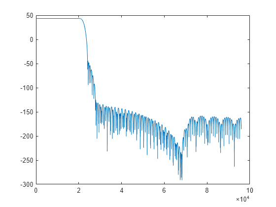
Create a multistage sample rate converter with default properties, corresponding to the combined three filter stages used to convert from 192 kHz to 44.1 kHz. Compute and display the frequency response.

src = dsp.SampleRateConverter;
[H,f] = freqz(src);
plot(f,20*log10(abs(H)))

Compute and display the frequency response over the range between 20 Hz and 44.1 kHz.

f = 20:10:44.1e3;
[H,f] = freqz(src,f);
plot(f,20*log10(abs(H)))

Create src, a multistage sample rate converter with default properties. src converts between 192 kHz and 44.1 kHz. Find the individual filters that are cascaded together to perform the conversion.

src = dsp.SampleRateConverter;
c = getFilters(src);

Visualize the frequency response of the decimator used in the first stage of the process.

m = c.Stage1;

[h,w] = freqz(m);
plot(w/pi,20*log10(abs(h)))
xlabel('\omega / \pi')
ylabel('Magnitude (dB)')

Create a multistage sample rate converter with default properties, corresponding to the combined three filter stages used to convert from 192 kHz to 44.1 kHz.

src = dsp.SampleRateConverter

src = 
  dsp.SampleRateConverter with properties:

        InputSampleRate: 192000
       OutputSampleRate: 44100
    OutputRateTolerance: 0
              Bandwidth: 40000
    StopbandAttenuation: 80

Display information about the design.

info(src)

ans = 
    'Overall Interpolation Factor    : 147
     Overall Decimation Factor       : 640
     Number of Filters               : 3
     Multiplications per Input Sample: 27.667188
     Number of Coefficients          : 8631
     Filters:                         
        Filter 1:
        dsp.FIRDecimator     - Decimation Factor   : 2 
        Filter 2:
        dsp.FIRDecimator     - Decimation Factor   : 2 
        Filter 3:
        dsp.FIRRateConverter - Interpolation Factor: 147
                             - Decimation Factor   : 160 
     '

Get the actual output sample rate for conversion between 192 kHz and 44.1 kHz when given a tolerance of 1%.

src = dsp.SampleRateConverter;
src.OutputRateTolerance = 0.01;
FsOut = getActualOutputRate(src)

FsOut = 
4.4308e+04

Create src, a multistage sample rate converter with default properties. src combines three filter stages to convert from 192 kHz to 44.1 kHz. Determine its overall interpolation and decimation factors.

src = dsp.SampleRateConverter;
[L,M] = getRateChangeFactors(src)

L = 
147

M = 
640

Create a multistage sample rate converter with default properties, corresponding to the combined three filter stages used to convert from 192 kHz to 44.1 kHz. Visualize the stages.

src = dsp.SampleRateConverter;
visualize(src)