Frequency-Domain FIR Filter
Filter input signal in the frequency domain
Libraries:
DSP System Toolbox /
Filtering /
Filter Implementations
Description
The Frequency-Domain FIR Filter block implements frequency-domain, fast
Fourier transform (FFT)-based filtering to filter a streaming input signal. In the time
domain, the filtering operation involves a convolution between the input and the impulse
response of the finite impulse response (FIR) filter. In the frequency domain, the
filtering operation involves the multiplication of the Fourier transform of the input
and the Fourier transform of the impulse response. The frequency-domain filtering
becomes more efficient than time-domain filtering as the impulse response grows longer.
You can specify the filter coefficients directly in the frequency domain by setting
Numerator domain to
Frequency.
This block uses the overlap-save and overlap-add methods to perform the frequency-domain filtering. For filters with a long impulse response length, the latency inherent to these two methods can be significant. To mitigate this latency, the Frequency-Domain FIR Filter block partitions the impulse response into shorter blocks and implements the overlap-save and overlap-add methods on these shorter blocks. To partition the impulse response, select the Partition numerator to reduce latency check box. For more details on these two methods and on reducing latency through impulse response partitioning, see Algorithms.
The Frequency-Domain FIR Filter block can model single-input multiple-output (SIMO) and multiple-input multiple-output (MIMO) systems by supporting multiple filters in the time domain and the frequency domain. For examples that show how to model such systems, see Filter Input Signal Using 1-by-2 SIMO System and Filter Input Signal Using 3-by-2 MIMO System. You can also specify multiple paths between each input channel and output channel pair using the Number of propagation paths parameter. For more information on modeling MIMO systems, see Modeling MIMO System with Multiple Propagation Paths. (since R2024a)
Examples
Filter input signal using the overlap-save and overlap-add methods and compare the filter output with the output of a time-domain FIR filter.
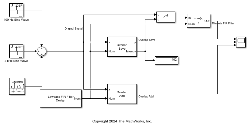
Open the overlapAddSave.slx model. The Lowpass FIR Filter Design block in the model designs the lowpass FIR filter with a filter order of 400 and a cutoff frequency of 0.5 in normalized frequency units. Use the Discrete FIR Filter block and the two Frequency-Domain FIR Filter blocks to filter the input signal using these coefficients.
The input signal in the model is a noisy sinusoidal signal with two tones, one at 100 Hz and the other at 3 kHz. The signal has a sample rate of 8000 Hz and a frame size of 256. The noise is a white Gaussian noise with a mean of 0 and a variance of 0.01.
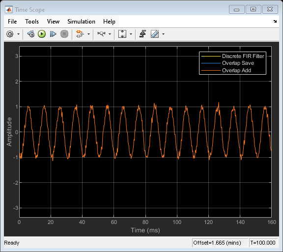
Pass the input signal to the three filters. Account for the output latency of the frequency-domain FIR filters while passing the input to the time-domain FIR filter. View the filtered outputs in the time scope.
Run the model. The outputs of all the three filters match exactly.
Partition the impulse response length of a frequency-domain FIR filter. Compare the outputs of the partitioned filter and the original filter.
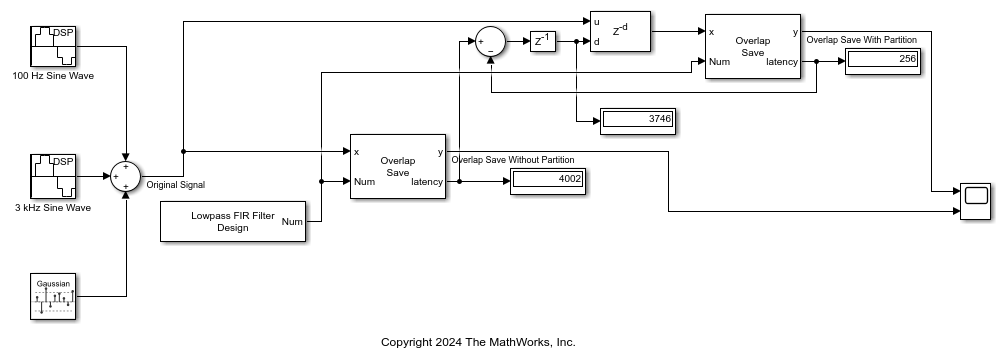
Open the reduceLatency.slx model. The Lowpass FIR Filter Design block in the model designs the lowpass FIR filter with a filter order of 4000 and a cutoff frequency of 0.5 in normalized frequency units. Use Frequency-Domain FIR Filter blocks to filter the input signal using these coefficients.
The input signal in the model is a noisy sinusoidal signal with two tones, one at 100 Hz and the other at 3 kHz. The signal has a sample rate of 8000 Hz and a frame size of 256. The noise is a white Gaussian noise with a mean of 0 and a variance of 0.01. Pass this data through the two frequency-domain filters.
Select the Partition numerator to reduce latency parameter in one of the Frequency-Domain FIR Filter blocks. Set the partition length to 256.
The latency of the frequency-domain FIR filter is given by  . By default, the FFT length is equal to twice the numerator length. This makes the latency proportional to the impulse response length. For the frequency-domain FIR filter with no partition, the latency is 4002 samples, and for the frequency-domain FIR filter with partition, the latency is 256 samples.
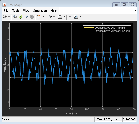
Run the model. Compare the outputs of the two frequency-domain filters in the time scope. To compare the two outputs, delay the input to the partitioned frequency-domain FIR filter by 3746 samples (4002  256). As you can see in the time scope, the outputs match exactly.
Specify the numerator coefficients of the frequency-domain FIR filter in the frequency domain. Filter the input signal using the overlap-add method. Compare the frequency-domain FIR filter output to the corresponding time-domain FIR filter output.
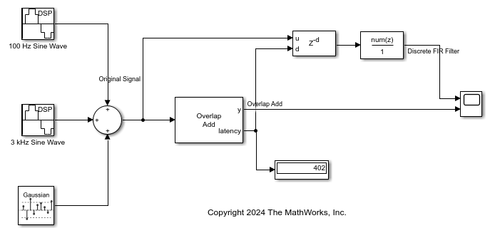
Open the specifyFrequencyResponse.slx model. The input is a noisy sinusoidal signal with two tones, one at 100 Hz and the other at 3 kHz. The noise is a white Gaussian noise with a mean of 0 and a variance of 0.01. Pass this signal to the Frequency-Domain FIR Filter block and the Discrete FIR Filter block.
Design the FIR lowpass filter coefficients using the designLowpassFIR function. The sampling frequency is 8 kHz, and the cutoff frequency of the filter is 2 kHz. Specify the time-domain impulse response in the Discrete FIR Filter block. Compute the FFT of this impulse response and specify this response as the frequency response of the frequency-domain FIR filter. In the Frequency-Domain FIR Filter block, set the time-domain numerator length to the number of elements in the time-domain impulse response.
Here is the MATLAB® code to design the filter.
order = 400;
Fs = 8000;
Fcutoff = 2000;
imp = designLowpassFIR(FilterOrder=order,CutoffFrequency=2*Fcutoff/Fs);
H = fft(imp,2*numel(imp));
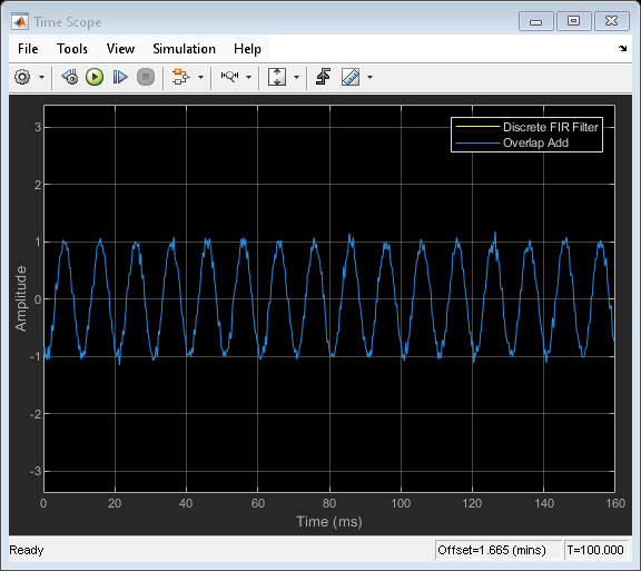
Run the model and visualize the frequency-domain FIR filter output and the time-domain FIR filter output in the time scope. To compare the outputs, delay the time-domain FIR filter input by the latency of the frequency-domain FIR filter.
The outputs of both the filters match exactly.
Since R2024a
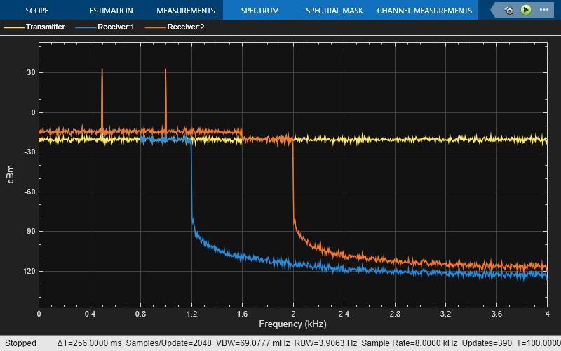
Filter an input signal using a 1-by-2 SIMO system with two distinct paths between the input and each output. Partition the filters to reduce latency.
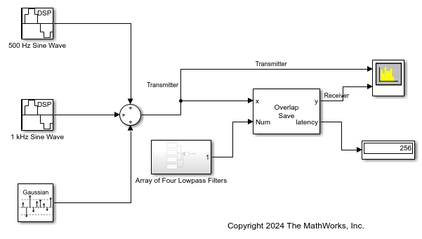
Open the filterSignalSIMOSystem.slx model. Design four lowpass FIR filters with different cutoff frequencies and concatenate the coefficients along the first dimension. The order for each filter is 4000 and the sampling rate is 8000 Hz. The SIMO system models one input channel, two output channels, and two paths between each input channel and output channel pair.
Pass the filter coefficients you design through the Num port of the Frequency-Domain FIR Filter block. Set the partition length of the filter to 256 and the number of propagation paths to 2. The block uses the Overlap-save method by default.
The input contains two sinusoidal signals each with a frame length of 256. The input noise is white Gaussian with a mean of 0 and a variance of 0.01. The first sinusoidal signal has a frequency of 500 Hz and the second sinusoidal signal has a frequency of 1000 Hz.
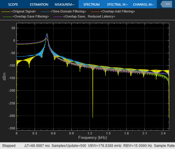
Run the model. Pass the signal through the designed filter. View the spectrum of the input and the filtered output in the spectrum analyzer.
Since R2024a
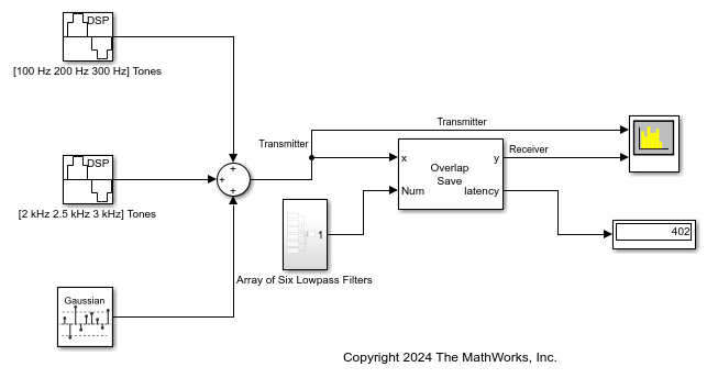
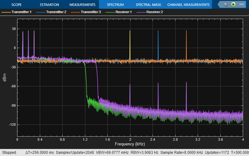
Filter an input signal using a 3-by-2 MIMO system with three input channels, two output channels, and one path between each input channel and output channel pair.
Open the filterSignalMIMOSystem.slx model. Design six lowpass FIR filters with different cutoff frequencies. The order for each filter is 400 and the sampling rate is 8000 Hz.
Pass the filter coefficients you design through the Num port of the Frequency-Domain FIR Filter block. The block uses the Overlap-save method by default. Select the Sum filtered output contributions from all input channels parameter.
The input contains two sinusoidal signals each with a frame length of 256. The first sinusoidal signal contains tones at 100 Hz, 200 Hz, and at 300 Hz. The second sinusoidal signal contains tones at 2 kHz, 2.5 kHz, and at 3 kHz. The input noise is white Gaussian with a mean of 0 and a variance of 0.01.
Run the model. Pass the signal through the designed filter. View the spectrum of the input and the filtered output in the spectrum analyzer.
Extended Examples
Overlap-Add/Save
Filter a sinusoid with the Overlap-Add and Overlap-Save FFT methods using the Frequency-Domain FIR filter block.
Ports
Input
Data input, specified as a vector or a matrix of size L-by-T. This block supports variable-size input signals, that is, you can change the input frame size (number of rows) even after calling the algorithm. However, the number of channels (number of columns) must remain constant.
This port is unnamed until you select the Specify coefficients from input port parameter.
Data Types: single | double
Complex Number Support: Yes
Specify the time-domain FIR filter coefficients as a row vector (single filter) or a matrix (multiple filters) (since R2024a) of size F-by-NumLen, where F is the number of filters and NumLen is the filter length. If F is greater than 1, then its value must be a multiple of the product of the number of input channels (columns) T and the number of paths P you specify through the Number of propagation paths parameter. The multiplication factor determines the number of output channels R and equals F/(T × P).
The coefficient values can change during simulation but the size of the numerator must remain constant.
Dependencies
To enable this port, set Numerator domain to
Time and select the Specify
coefficients from input port parameter.
Data Types: single | double | int8 | int16 | int32 | uint8 | uint16 | uint32
Complex Number Support: Yes
Specify the frequency-domain FIR filter coefficients as a row vector, matrix, or a 3-D array (since R2024a).
When you clear the Partition numerator to reduce latency parameter, the coefficients input at this port can be a row vector or a matrix of size F-by-FFTLength. The FFT length is equal to the length of the vector input. If F is greater than 1 (multiple filters) (since R2024a), then its value must be a multiple of the product of the number of input channels (columns) T and the number of paths P you specify through the Number of propagation paths parameter. The multiplication factor determines the number of output channels R and equals F/(T × P).
When you select the Partition numerator to reduce latency parameter, Frequency response must be a matrix of size 2PL-by-N to represent a single filter or a 3-D array (since R2024a) of size 2PL-by-N-by-F to represent multiple filters, where PL is the partition size, N is the number of partitions, and F is the number of filters.
Dependencies
To enable this port, set Numerator domain to
Frequency and select the Specify
frequency response from input port parameter.
Data Types: single | double | int8 | int16 | int32 | uint8 | uint16 | uint32
Complex Number Support: Yes
Output Arguments
Filtered output, returned as a vector, matrix or a 3D array (since R2024a).
When the number of filters F is greater than 1 and you select the Sum filtered output contributions from all input channels parameter, the block adds the filtered output from each input channel to generate an L-by-R output matrix, where L is the input frame size (number of input rows) and R is the number of output channels. R equals F/(T x P), where F is the number of filters, T is the number of input channels, and P is the value that you specify in the Number of propagation paths parameter. (since R2024a)
When you clear the Sum
filtered output contributions from all input channels
parameter, the block does not sum filtered output contributions from all
input channels. The output is an
L-by-R-by-T
array. output(:,j,k) refers to the output from the
kth input channel for
the jth output channel.
For example, output(:,3,2) indicates output on the
third output channel from the second input channel. (since R2024a)
For more information on how the object computes the output, see Algorithms.
The output has the same data type and complexity as the input signal.
This port is unnamed until you select the Output filter latency parameter and click Apply.
Data Types: single | double
Complex Number Support: Yes
Filter latency, returned as a scalar. This latency is inherent to overlap-add and overlap-save methods and does not include the group delay of the filter. This port appears only when you select the Output filter latency check box.
This port is unnamed until you select the Output filter latency check box and click Apply.
Data Types: uint32
Parameters
Specify the filtering method in the frequency domain as
Overlap-save or
Overlap-add. For more details on these two
methods, see Algorithms.
Specify the domain of the filter coefficients as one of the following:
Time— Specify the time-domain filter coefficients in the Filter coefficients parameter or through the Num input port.Frequency— Specify the filter's frequency response in the Frequency response parameter or through the NumFFT input port.
When you select this check box, the time-domain FIR filter coefficients are input through the port, Num. When you clear this check box, the coefficients are specified in the block dialog box through the Filter coefficients parameter.
To view the filter response, clear this check box, specify the coefficients in the block dialog box, and click on the View Filter Response button.
Dependencies
To enable this parameter, set Numerator domain to
Time.
Specify the time-domain FIR filter coefficients as a row vector (single filter) or a matrix (multiple filters) (since R2024a) of size F-by-NumLen, where F is the number of filters and NumLen is the filter length. If F is greater than 1, then its value must be a multiple of the product of the number of input channels (columns) T and the number of paths P you specify through the Number of propagation paths parameter. The multiplication factor determines the number of output channels R and equals F/(T × P).
The coefficient values can change during simulation but the size of the numerator must remain constant.
Tunable: Yes
Dependencies
To enable this parameter, set Numerator domain to
Time and clear the Specify
coefficients from input port parameter.
Data Types: single | double | int8 | int16 | int32 | int64 | uint8 | uint16 | uint32 | uint64
Complex Number Support: Yes
When you select this check box, the FIR filter coefficients in the frequency domain are input through the port, NumFFT. When you clear this check box, the coefficients are specified in the block dialog box through the Frequency response parameter.
To view the filter response, clear this check box, specify the frequency response in the block dialog box, and click on the View Filter Response button.
Dependencies
To enable this parameter, set Numerator domain to
Frequency.
Specify the frequency response of the filter as a row vector, matrix, or a 3-D array (since R2024a).
When you clear the Partition numerator to reduce latency parameter, Frequency response can be a row vector or a matrix of size F-by-FFTLength. The FFT length is equal to the length of the Frequency response vector. If F is greater than 1 (multiple filters) (since R2024a), then its value must be a multiple of the product of the number of input channels (columns) T and the number of paths P you specify through the Number of propagation paths parameter. The multiplication factor determines the number of output channels R and equals F/(T × P).
When you select the Partition numerator to reduce latency parameter, Frequency response must be a matrix of size 2PL-by-N to represent a single filter or a 3-D array (since R2024a) of size 2PL-by-N-by-F to represent multiple filters, where PL is the partition size, N is the number of partitions, and F is the number of filters.
Tunable: Yes
Dependencies
To enable this parameter, set Numerator domain to
Frequency and clear the Specify
frequency response from input port parameter.
Data Types: single | double | int8 | int16 | int32 | uint8 | uint16 | uint32
Complex Number Support: Yes
Since R2024a
Specify the number of propagation paths P between each
input channel and output channel pair as a positive integer. Each path is
represented by a unique filter. When you specify the number of paths to be
greater than 1, the filter models multipath propagation.
The algorithm sums up the filtered output contributions from all paths
between each input channel and output channel pair.
For an example, see Filter Input Signal Using 1-by-2 SIMO System.
Dependencies
To enable this parameter, the number of filters F must be greater than 1.
Data Types: single | double
Since R2024a
Select this check box to sum filtered output contributions from all input channels. When you select this check box, the block adds the filtered output from each input channel to generate an L-by-R output matrix, where L is the input frame size (number of input rows) and R is the number of output channels. R equals F/(T x P), where F is the number of filters, T is the number of input channels, and P is the value that you specify through the Number of propagation paths parameter.
When you clear this parameter, the block does not sum filtered output contributions from all input channels. The output is an L-by-R-by-T array.
For more information on how the block computes the output based on the value of this parameter, see Modeling MIMO System with Multiple Propagation Paths.
Dependencies
To enable this property, the number of filters F must be greater than 1.
Select this parameter to partition the numerator to reduce latency. When you select this parameter, the block partitions the numerator into segments of length specified by the Numerator partition length parameter. The filter performs overlap-save or overlap-add on each partition, and combines the partial results to form the overall output. This option reduces latency to the partition length.
When you clear this parameter, the filter uses the traditional overlap-save or overlap-add method. The latency in this case is FFT length – NumLen + 1, where NumLen is the filter length. See the Filter coefficients parameter for more information on the filter length.
Specify the partition length of the numerator PL as a positive integer less than or equal to the length of the numerator.
Dependencies
To enable this parameter, set Numerator domain to
Time and select the Partition
numerator to reduce latency parameter.
Data Types: single | double | int8 | int16 | int32 | int64 | uint8 | uint16 | uint32 | uint64
Specify the time-domain numerator length as a positive integer.
Dependencies
To enable this parameter, set Numerator domain to
Frequency and clear the
Partition numerator to reduce latency check
box.
Data Types: single | double | int8 | int16 | int32 | uint8 | uint16 | uint32
When you select this check box, the FFT length equals twice the numerator length. When you clear this check box, you specify the FFT length through the FFT length parameter.
Dependencies
To enable this parameter, set Numerator domain to
Time and clear the Partition
numerator to reduce latency parameter.
The FFT length you specify must be greater than or equal to the length of the numerator you specify in the Filter coefficients parameter.
Dependencies
To enable this parameter, set Numerator domain to
Time, clear the Partition
numerator to reduce latency and the Inherit FFT
length from numerator length parameters.
Data Types: single | double | int8 | int16 | int32 | int64 | uint8 | uint16 | uint32 | uint64
Select this parameter to specify that the filter coefficients are all real.
Dependencies
To enable this parameter, set Numerator domain to
Frequency.
When you select this check box and click Apply, the block outputs the filter latency through the latency port.
Clicking this button opens the filter visualizer and displays the magnitude response of the frequency domain FIR filter. The response is based on the parameters you select in the block dialog box. To update the response while the visualizer is running, modify the parameters in the dialog box and click Apply.
You can configure the plot settings and the frequency response measurements from the interface of the visualizer.
On the Scope tab, you can enable the legend, specify to plot both magnitude and phase responses of the filter, modify the plot settings, generate a script to re-create the plot, and even save or share the settings. On the Measurements tab, you can enable data cursors, and display the peak values of the filter response.
For more details on the filter visualizer interface and its tools, see Configure Filter Visualizer.
Dependencies
To enable this button, clear the Specify coefficients from input port and the Specify frequency response from input port parameters.
Specify the type of simulation to run. You can set this parameter to:
Interpreted execution— Simulate model using the MATLAB® interpreter. This option shortens startup time.Code generation— Simulate model using generated C code. The first time you run a simulation, Simulink® generates C code for the block. The C code is reused for subsequent simulations as long as the model does not change. This option requires additional startup time but provides faster subsequent simulations.
Block Characteristics
Data Types |
|
Direct Feedthrough |
|
Multidimensional Signals |
|
Variable-Size Signals |
|
Zero-Crossing Detection |
|
Algorithms
Overlap-save and overlap-add are the two frequency-domain FFT-based filtering methods this algorithm uses.
The overlap-save method is implemented using the following approach:

The input stream is partitioned into overlapping blocks of size FFTLen, with an overlap factor of NumLen – 1 samples. FFTLen is the FFT length and NumLen is the length of the FIR filter numerator. The FFT of each block of input samples is computed and multiplied with the length-FFTLen FFT of the FIR numerator. The inverse fast Fourier transform (IFFT) of the result is performed, and the last FFTLen – NumLen + 1 samples are saved. The remaining samples are dropped.
The latency of overlap-save is FFTLen – NumLen + 1. The first FFTLen – NumLen + 1 samples are equal to zero. The filtered value of the first input sample appears as the FFTLen – NumLen + 2 output sample.
Note that the FFT length must be larger than the numerator length, and is typically set to a value much greater than NumLen.
The overlap-add method is implemented using the following approach:

The input stream is partitioned into blocks of length FFLen – NumLen + 1, with no overlap between consecutive blocks. Similar to overlap-save, the FFT of the block is computed, and multiplied by the FFT of the FIR numerator. The IFFT of the result is then computed. The first NumLen + 1 samples are modified by adding the values of the last NumLen + 1 samples from the previous computed IFFT.
The latency of overlap-add is FFTLen – NumLen + 1. The first FFTLen – NumLen + 1 samples are equal to zero. The filtered value of the first input sample appears as the FFTLen – NumLen + 2 output sample.
With an FFT length that is twice the length of the FIR numerator, the latency roughly equals the length of the FIR numerator. If the impulse response is very long, the latency becomes significantly large. However, frequency domain FIR filtering is still faster than the time-domain filtering. To mitigate the latency and make the frequency domain filtering even more efficient, the algorithm partitions the impulse response into multiple short blocks and performs overlap-save or overlap-add on each block. The results of the different blocks are then combined to obtain the final output. The latency of this approach is of the order of the block length, rather than the entire impulse response length. This reduced latency comes at the cost of additional computation. For more details, see [1].
These diagrams present a generalized representation of a frequency-domain FIR filter using multiple filters to process signals between multiple input channels and output channels. This diagram models multiple paths between each input channel-output channel pair.
SumFilteredOutputs is
true
The algorithm passes the first input channel through the first set of R × P filters within which ((i − 1) × P + 1) to (i × P) filters compute the output for the ith output channel. The algorithm passes the second input channel through the next set of R × P filters, and the sequence continues until the last input channel passes through the filter F.
The algorithm adds the filtered output contributions from all input channels before sending them as the respective output channel.
The input signal is of size L-by-T.
L is the input frame size (number of input rows).
T is the number of input channels.
F is the number of filters. This value is the number of rows in the filter coefficients matrix.
Filter coefficients is a matrix of size F-by-numLen. Each row corresponds to a filter of length numLen.
P is the number of propagation paths between each input channel and output channel.
R is the number of output channels and equals F/(T x P).
Output signal is of size L-by-R. Each output channel is of size L-by-1.
SumFilteredOutputs is
false
The algorithm concatenates the filtered outputs and does not sum across input
channels. The output is an
L-by-R-by-T array that you
can further process before sending it to the output. For example, if you add elements in
the L-by-R-by-T array across
the third dimension, the resultant L-by-R array is
same as the output signal you get when you set SumFilteredOutputs
to true.
References
[1] Stockham, T. G., Jr. "High Speed Convolution and Correlation." Proceedings of the 1966 Spring Joint Computer Conference, AFIPS, 28 (1966): 229–233.
Extended Capabilities
C/C++ Code Generation
Generate C and C++ code using Simulink® Coder™.
Version History
Introduced in R2017bThe default value of the Simulate using parameter is now
Interpreted execution. With this change, the block uses the
MATLAB interpreter for simulation by default.
You can model MIMO systems by specifying multiple filters in the time and frequency domains. You can also specify multiple paths between each input and output pair.
MATLAB Command
You clicked a link that corresponds to this MATLAB command:
Run the command by entering it in the MATLAB Command Window. Web browsers do not support MATLAB commands.
选择网站
选择网站以获取翻译的可用内容,以及查看当地活动和优惠。根据您的位置,我们建议您选择:。
您也可以从以下列表中选择网站:
如何获得最佳网站性能
选择中国网站(中文或英文)以获得最佳网站性能。其他 MathWorks 国家/地区网站并未针对您所在位置的访问进行优化。
美洲
- América Latina (Español)
- Canada (English)
- United States (English)
欧洲
- Belgium (English)
- Denmark (English)
- Deutschland (Deutsch)
- España (Español)
- Finland (English)
- France (Français)
- Ireland (English)
- Italia (Italiano)
- Luxembourg (English)
- Netherlands (English)
- Norway (English)
- Österreich (Deutsch)
- Portugal (English)
- Sweden (English)
- Switzerland
- United Kingdom (English)
