dsp.FrequencyDomainAdaptiveFilter

Compute output, error, and coefficients using frequency-domain FIR adaptive filter

Description

The dsp.FrequencyDomainAdaptiveFilter System object™ implements an adaptive finite impulse response (FIR) filter in the frequency domain using the fast block least mean squares (LMS) algorithm. The Length and the BlockLength properties specify the filter length and the block length values the algorithm uses. The FFTCoefficients property contains the discrete Fourier transform of the current filter coefficients. The object offers the constrained and unconstrained versions of the algorithm with partitioned and non-partitioned modes. For details, see Algorithms.

To filter a signal using frequency-domain FIR adaptive filter:

Create the dsp.FrequencyDomainAdaptiveFilter object and set its properties.
Call the object with arguments, as if it were a function.

To learn more about how System objects work, see What Are System Objects?

Creation

Syntax

fdaf = dsp.FrequencyDomainAdaptiveFilter

fdaf = dsp.FrequencyDomainAdaptiveFilter(len)

fdaf = dsp.FrequencyDomainAdaptiveFilter(___,Name,Value)

Description

fdaf = dsp.FrequencyDomainAdaptiveFilter returns a frequency domain FIR adaptive filter System object, fdaf. This System object is used to compute the filtered output and the filter error for a given input and desired signal.

example

fdaf = dsp.FrequencyDomainAdaptiveFilter(len) returns a frequency domain FIR adaptive filter object with the Length property set to len.

example

fdaf = dsp.FrequencyDomainAdaptiveFilter(___,Name,Value) returns a frequency domain FIR adaptive filter object with each specified property set to the specified value. Enclose each property name in quotes. You can use this syntax with any previous input argument combinations.

Example: fdaf = dsp.FrequencyDomainAdaptiveFilter('Length',32,'StepSize',0.1) models a frequency-domain adaptive filter with a length of 32 taps and a step size of 0.1.

example

Properties

expand all

Unless otherwise indicated, properties are nontunable, which means you cannot change their values after calling the object. Objects lock when you call them, and the release function unlocks them.

If a property is tunable, you can change its value at any time.

For more information on changing property values, see System Design in MATLAB Using System Objects.

`Method` — Method to calculate filter coefficients
`'Constrained FDAF'` (default) | `'Unconstrained FDAF'` | `'Partitioned constrained FDAF'` | `'Partitioned unconstrained FDAF'`

Method used to calculate the filter coefficients, specified as:

'Constrained FDAF' –– Imposes a gradient constraint on the filter tap weights.
'Unconstrained FDAF' –– No gradient constraint is imposed on the filter tap weights.
'Partitioned constrained FDAF' –– Partitions the impulse response of the filter to reduce latency.
'Partitioned unconstrained FDAF' –– Partitions the impulse response of the filter to reduce latency. No gradient constraint is imposed on the filter tap weights.

For more details, see Algorithms.

`Length` — Length of filter coefficients vector
`32` (default) | positive, integer-valued scalar

Length of the FIR filter coefficients vector, specified as a positive, integer-valued scalar.

`BlockLength` — Block length for coefficient updates
`32` (default) | positive, integer-valued scalar

Block length for the coefficient updates, specified as a positive, integer-valued scalar. The adaptive filter processes the input data and the desired signal as a block of samples of length set by this property. For details on how this data is processed by the filter, see Algorithms. The length of the input vector must be divisible by the BlockLength property value. The default value of the BlockLength property is set to the value of the Length property.

`StepSize` — Adaptation step size
`1` (default) | real scalar in the range (0,1]

Adaptation step size factor, specified as a real scalar in the range (0,1]. Using a small step size ensures a small steady-state error. However, a small step size decreases the resulting convergence speed of the adaptive filter. Increasing the step size improves the convergence speed, at the cost of increased steady-state mean squared error. When the step size value is 1, the algorithm provides the optimal tradeoff between the convergence speed and the steady-state mean squared error.

Tunable: Yes

`LeakageFactor` — Adaptation leakage factor
`1` (default) | scalar in the range [0,1]

Leakage factor used when implementing a leaky adaptive filter, specified as a scalar numeric value in the range [0,1]. When the value is less than 1, the System object implements a leaky adaptive algorithm. When the value is 1, the object provides no leakage in the adapting method.

Tunable: Yes

`AveragingFactor` — Averaging factor for signal power
`0.9` (default) | real scalar in the range (0,1]

Averaging factor used to compute the exponentially windowed FFT input signal powers for the coefficient updates, specified as a real scalar in the range (0,1].

Tunable: Yes

`Offset` — Offset for normalization terms
`0` (default) | nonnegative real scalar

Offset for the normalization terms in the coefficient updates, specified as a nonnegative real scalar value. This property value is used to avoid division by zero or division by very small numbers if any of the FFT input signal powers become very small.

Tunable: Yes

`InitalPower` — Initial FFT input signal power
`1` (default) | positive numeric scalar

Initial common value of all of the FFT input signal powers, specified as a positive numeric scalar.

If you change this value once the object is locked, the change takes effect only after you reset the object.

Tunable: Yes

`InitialCoefficients` — Initial time-domain coefficients of filter
`0` (default) | scalar | vector

Initial time-domain coefficients of the adaptive filter, specified as a scalar or a vector of length equal to the Length property value. The adaptive filter object uses these coefficients to compute the initial frequency-domain filter coefficients.

If you change this value once the object is locked, the change takes effect only after you reset the object.

Tunable: Yes

`LockCoefficients` — Locked status of coefficient updates
`false` (default) | `true`

Locked status of the coefficient updates, specified as:

false –– The object continuously updates the filter coefficients.
true –– The filter coefficients do not get updated and their values remain at the current value.

Tunable: Yes

Data Types: logical

`FFTCoefficients` — Current FFT coefficients of filter
`[]` (default) | row vector

This property is read-only.

Current discrete Fourier transform of the filter coefficients, returned as a row vector. For 'Constrained FDAF' and 'Unconstrained FDAF' algorithms, the length of this vector is equal to the sum of the Length value and the BlockLength value. This property is initialized to the FFT values of the InitialCoefficients property. To get the discrete Fourier transform of the filter coefficients, call the object, and access the FFTCoefficients property of the object.

Data Types: single | double
Complex Number Support: Yes

Usage

Syntax

[y,err] = fdaf(x,d)

Description

[y,err] = fdaf(x,d) filters the input signal, x, using d as the desired signal, and returns the filtered output in y and the filter error in err. The System object estimates the filter weights needed to minimize the error between the output signal and the desired signal. The FFT of these filter weights can be obtained by accessing the FFTCoefficients property after calling the object algorithm.

Input Arguments

expand all

`x` — Data input
column vector

The signal to be filtered by the frequency-domain FIR adaptive filter. The input, x, and the desired signal, d, must have the same size and data type. The length of the input vector must be divisible by the BlockLength property value.

The input, x, can be a variable-size signal as long as the frame length is a multiple of the BlockLength. You can change the number of elements in the column vector even when the object is locked. The System object locks when you call the object to run its algorithm.

Data Types: single | double
Complex Number Support: Yes

`d` — Desired signal
column vector

The frequency domain adaptive filter adapts its filter weights to minimize the error, err, and converge the input signal, x, to the desired signal, d, as closely as possible.

The input signal and the desired signal must have the same size and data type. The length of the desired signal vector must be divisible by the BlockLength property value.

The input signal can be a variable-size signal as long as the frame length is a multiple of the BlockLength. You can change the number of elements in the column vector even when the object is locked. The System object locks when you call the object to run its algorithm.

Data Types: single | double
Complex Number Support: Yes

Output Arguments

expand all

`y` — Filtered output
column vector

Filtered output, returned as a column vector. The object adapts its filter weights to converge the input signal, x, to match the desired signal, d. The filter outputs the converged signal.

Data Types: single | double
Complex Number Support: Yes

`err` — Difference between output and desired signal
column vector

Difference between the output signal and the desired signal, returned as a column vector. The objective of the adaptive filter is to minimize this error. The object adapts its weights to converge towards optimal filter weights which produce an output signal that matches the desired signal as closely as possible. For more details on how err is computed, see [2].

Data Types: single | double
Complex Number Support: Yes

Object Functions

To use an object function, specify the System object as the first input argument. For example, to release system resources of a System object named obj, use this syntax:

release(obj)

expand all

Common to All System Objects

`step`	Run System object algorithm
`release`	Release resources and allow changes to System object property values and input characteristics
`reset`	Reset internal states of System object

Examples

collapse all

QPSK Adaptive Equalization With FIR Filter

Open Live Script

Transmit a quadrature phase shift keying (QPSK) signal across a noisy transmission channel. Minimize the noise in the received signal using a frequency-domain adaptive filter.

The QPSK signal, s, is transmitted across a noisy channel. The numerator and the denominator coefficients of the channel are contained in the vectors b and a, respectively. The received signal, r, obtained at the end of the transmission channel contains the transmitted QPSK signal and the noise added to the channel, n. The adaptive filter is used to extract the QPSK signal from the received noisy input. The desired signal, d, is the delayed version of the QPSK signal.

D = 16;
b  = exp(1i*pi/4)*[-0.7 1];
a  = [1 -0.7];
ntr = 1024;
s  = sign(randn(1,ntr+D)) + 1i*sign(randn(1,ntr+D));
n  = 0.1*(randn(1,ntr+D) + 1i*randn(1,ntr+D));
r  = filter(b,a,s) + n;
x  = r(1+D:ntr+D);
d  = s(1:ntr);

Create a dsp.FrequencyDomainAdaptiveFilter object to model a frequency-domain adaptive filter of length 32 taps and a step size of 0.1. The adaptive filter accepts the delayed version of the received signal and the desired signal as inputs. The output of the adaptive filter is compared to the desired signal. The error between the two signals represents the noise added to the transmission channel. The adaptive filter updates its coefficients until this error becomes minimal. To get the discrete Fourier transform of the filter coefficients, call the fdaf object, and access the FFTCoefficients property of this object.

mu  = 0.1;
fdaf = dsp.FrequencyDomainAdaptiveFilter('Length',32,'StepSize',mu);
[y,e] = fdaf(x,d);
fftCoeffs = fdaf.FFTCoefficients

fftCoeffs = 1×64 complex

   0.6802 - 0.6847i  -0.2485 - 0.9427i  -0.9675 - 0.2123i  -0.5605 + 0.8002i   0.5748 + 0.7593i   0.8541 - 0.3917i  -0.2526 - 0.9022i  -0.9298 + 0.1255i   0.0181 + 0.9366i   0.9207 + 0.0511i   0.1063 - 0.8972i  -0.8919 - 0.1829i  -0.2668 + 0.9113i   0.9215 + 0.3186i   0.3417 - 0.8859i  -0.8285 - 0.3760i  -0.4317 + 0.8200i   0.8741 + 0.4765i   0.4874 - 0.9075i  -0.8517 - 0.4774i  -0.4709 + 0.7632i   0.7468 + 0.4833i   0.5193 - 0.7995i  -0.8218 - 0.5649i  -0.5908 + 0.7768i   0.7316 + 0.5866i   0.5806 - 0.7270i  -0.7148 - 0.5998i  -0.6287 + 0.6702i   0.6575 + 0.6379i   0.6332 - 0.7153i  -0.7659 - 0.6424i  -0.6678 + 0.7294i   0.6536 + 0.6891i   0.7006 - 0.6333i  -0.6594 - 0.7117i  -0.7207 + 0.6517i   0.6031 + 0.7239i   0.7362 - 0.5776i  -0.5869 - 0.7682i  -0.7975 + 0.5789i   0.5449 + 0.7992i   0.7909 - 0.5343i  -0.5512 - 0.8070i  -0.8392 + 0.5338i   0.4605 + 0.8493i   0.8358 - 0.3921i  -0.3751 - 0.8388i  -0.8739 + 0.3785i   0.3625 + 0.9048i

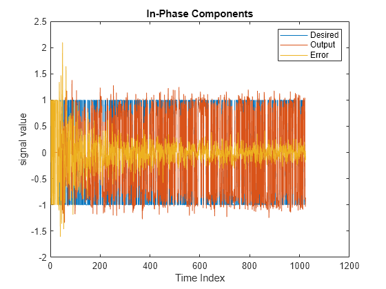
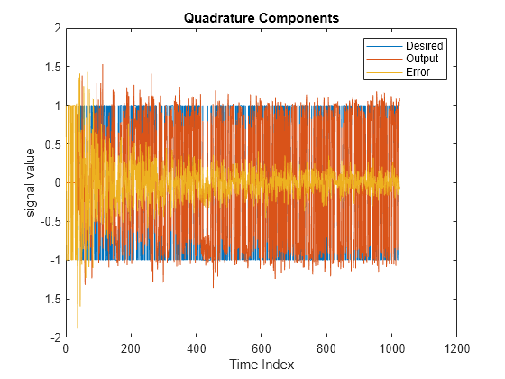
Plot the In-Phase and the Quadrature components of the desired, output, and the error signals.

plot(1:ntr,real([d;y;e]))
legend('Desired','Output','Error')
title('In-Phase Components')
xlabel('Time Index'); ylabel('signal value')

Figure contains an axes object. The axes object with title In-Phase Components, xlabel Time Index, ylabel signal value contains 3 objects of type line. These objects represent Desired, Output, Error.

plot(1:ntr,imag([d;y;e]))
legend('Desired','Output','Error')
title('Quadrature Components')
xlabel('Time Index')
ylabel('signal value')

Figure contains an axes object. The axes object with title Quadrature Components, xlabel Time Index, ylabel signal value contains 3 objects of type line. These objects represent Desired, Output, Error.

Create scatter plots of the received signal and the desired signal.

plot(x(ntr-100:ntr),'.')
axis([-3 3 -3 3])
title('Received Signal Scatter Plot')
axis('square')
xlabel('Real[x]')
ylabel('Imag[x]') 
grid on

Figure contains an axes object. The axes object with title Received Signal Scatter Plot, xlabel Real[x], ylabel Imag[x] contains a line object which displays its values using only markers.

plot(d(ntr-100:ntr),'.')
axis([-3 3 -3 3])
title('Desired Signal Scatter Plot')
axis('square')
xlabel('Real[y]')
ylabel('Imag[y]')
grid on

Figure contains an axes object. The axes object with title Desired Signal Scatter Plot, xlabel Real[y], ylabel Imag[y] contains a line object which displays its values using only markers.

The adaptive filter equalizes the received signal to eliminate noise. Plot the scatter plot of the equalized signal.

plot(y(ntr-100:ntr),'.')
axis([-3 3 -3 3])
title('Equalized Signal Scatter Plot')
axis('square')
xlabel('Real[y]')
ylabel('Imag[y]')
grid on

Figure contains an axes object. The axes object with title Equalized Signal Scatter Plot, xlabel Real[y], ylabel Imag[y] contains a line object which displays its values using only markers.

Estimate Coefficients of long FIR Filter using Frequency-Domain Adaptive Filter

Open Script

Use a frequency-domain adaptive filter to estimate the coefficients of a long FIR filter. The FIR filter models the impulse response of a room. Use the partitioned mode in the frequency-domain adaptive filter to reduce filter latency.

Note: This example runs only in R2018a or later.

Initialization

Generate a long FIR impulse response of 8192 samples and assign the impulse response to a dsp.FIRFilter object, room. This object models the impulse response of a room. Create a dsp.FrequencyDomainAdaptiveFilter filter, lmsfilt, in partitioned constrained mode. Set the length of the filter to one-fourth the length of the impulse response of the room. Set the block length of the filter to 128 samples. Set the step size to 0.025, initial power to 0.01, averaging factor to 0.98, offset to 1, and the leakage factor to 1. Initialize a dsp.ArrayPlot object to view the filter coefficients. Initialize a timescope object to show the mean-squared error between the filter output and the desired signal.

fs = 16e3;
m = 8192;
[b,a] = cheby2(4,20,[0.1 0.7]);
impulseResponseGenerator = dsp.IIRFilter(...
    'Numerator', [zeros(1,6) b], ...
    'Denominator', a);
roomImpulseResponse = impulseResponseGenerator( ...
    (log(0.99*rand(1,m)+0.01).*sign(randn(1,m)).*exp(-0.002*(1:m)))');
roomImpulseResponse = roomImpulseResponse/norm(roomImpulseResponse);
room = dsp.FIRFilter('Numerator',roomImpulseResponse');

lmsfilt = dsp.FrequencyDomainAdaptiveFilter(...
    'Method','Partitioned constrained FDAF',...
    'Length',m/4, ...
    'BlockLength',128,...
    'StepSize',0.025, ...
    'InitialPower',0.01, ...
    'AveragingFactor',0.98,...
    'Offset',1,...
    'LeakageFactor',1);

FrameSize = lmsfilt.BlockLength; NIter = 2000;

AP = dsp.ArrayPlot('YLimits',[-0.2 .2],'ShowLegend',true, ...
    'Position',[0 0 560 420],'ChannelNames', ...
    {'Actual Coefficients','Estimated Coefficients'});

TS = timescope('SampleRate',fs,'TimeSpanSource','property',...
    'TimeSpan',FrameSize*NIter/fs,...
    'TimeUnits','Seconds',...
    'YLimits',[-50 0],'Title','Learning curve',...
    'YLabel','dB', ...
    'BufferLength',FrameSize*NIter,...
    'ShowGrid',true);

signalmean = dsp.MovingAverage('SpecifyWindowLength',false);

Streaming

Generate a random input signal using the randn function. The frame size of the input matches the block length of the adaptive filter. The desired signal is the sum of the output of the FIR filter (room) and a white Gaussian noise signal. Pass the input signal and the desired signal to the adaptive filter. Compute the adaptive filter output and the error between the output and the desired signal.

Estimate the time-domain coefficients of the adaptive filter by taking the IFFT of the frequency-domain coefficients vector returned by the lmsfilt.FFTCoefficients property. Compare the estimated coefficients with the actual coefficients assigned to the FIR filter (room). Once the adaptive filter has converged its output to the desired signal, and minimized the error signal, the estimated coefficients match closely with the actual coefficients. This means that the adaptive filter has successfully adapted itself to model the impulse response of the FIR filter (room).

for k = 1:NIter
    x = randn(FrameSize,1);
    d = room(x) + 0.01*randn(FrameSize,1);
    [y,e] = lmsfilt(x,d);
    FFTCoeffs = lmsfilt.FFTCoefficients;
    w = ifft(FFTCoeffs,[],2,'symmetric');
    w = w(:,1:FrameSize) + w(:,FrameSize+1:end);
    w = reshape(w.',1,m/4);
    AP([roomImpulseResponse(1:m/4),w.']);
    TS(10*log10(signalmean(abs(e).^2)));
end

As the filter adapts with time, you can see in the time scope that the mean-squared error becomes minimal. Simultaneously, the estimated coefficients match the actual coefficients closely in the array plot.

Algorithms

expand all

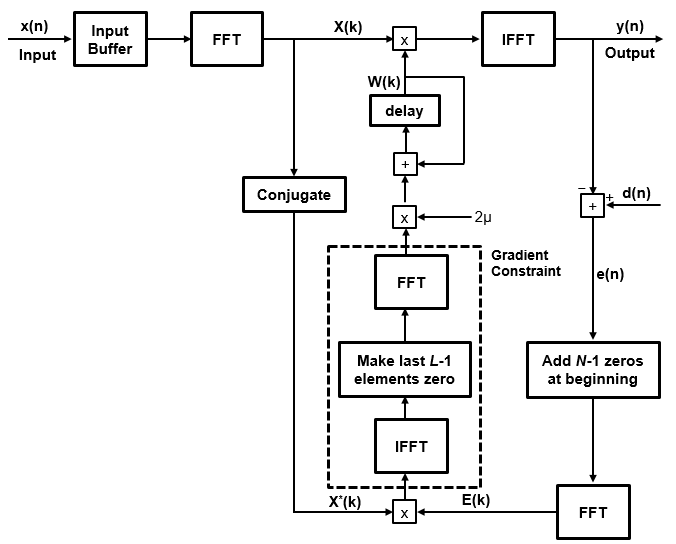
Frequency-domain adaptive filtering consists of three steps - filtering, error estimation, and tap-weight adaptation. This algorithm implements FIR filtering in the frequency domain using the overlap-save or overlap-add method. For more implementation details of these two methods, see the Algorithms section in the dsp.FrequencyDomainFIRFilter object page. The error estimation and the tap-weight adaptation are implemented using the fast block LMS algorithm (FBLMS).

Fast Block LMS Algorithm

The frequency-domain adaptive filter processes input data and the desired signal data as a block of samples using the fast block LMS (FBLMS) algorithm. Here is the block diagram of the frequency-domain adaptive filter using the FBLMS algorithm. The frequency-domain FIR filter in this diagram uses the overlap-save method.

where:

N –– Filter length
L –– Block length
μ –– Step size parameter
x(n) –– Input signal
X(k) –– Transformed input signal in the frequency domain
d(n) –– Desired signal
e(n) –– Error between the desired signal and the filter output
E(n) –– Transformed error signal in the frequency domain
W(k) –– Tap-weights vector in the frequency domain

For more details on how the error is estimated and the tap-weights are adapted, see [2].

Constrained and Unconstrained FBLMS Algorithms

The previous diagram is the constrained version. If you remove the gradient constraint portion of the algorithm, you have the unconstrained FBLMS implementation. For details on the convergence behavior of both constrained and unconstrained variations, see [2].

Partitioned FBLMS Algorithm

The latency of the filter roughly equals the length of the FIR numerator. If the impulse response of the filter is very long, the latency becomes significantly large. The partitioned FBLMS algorithm reduces latency by partitioning the impulse response. The nonpartitioned frequency-domain FIR filtering is faster than the time-domain filtering for long impulse responses, at the cost of increased latency. To mitigate the latency and make the frequency domain filtering even more efficient, the algorithm partitions the impulse response into multiple short blocks and performs overlap-save or overlap-add on each block. The results of the different blocks are then combined to obtain the final output. The latency of this approach is of the order of the block length, rather than the entire impulse response length. This reduced latency comes at the cost of additional computation. For more details on the implementation, see [2].

References

[1] Shynk, J.J. "Frequency-Domain and Multirate Adaptive Filtering." IEEE Signal Processing Magazine. Vol. 9, Number 1, 1992, pp. 14–37.

[2] Farhang-Boroujeny, B., Adaptive Filters: Theory and Applications, Chichester, England, Wiley, 1998.

[3] Stockham, T. G., Jr. "High Speed Convolution and Correlation." Proceedings of the 1966 Spring Joint Computer Conference, AFIPS, Vol. 28, 1966, pp. 229–233.

Extended Capabilities

C/C++ Code Generation
Generate C and C++ code using MATLAB® Coder™.

Usage notes and limitations:

System Objects in MATLAB Code Generation (MATLAB Coder).

Version History

Introduced in R2013b

dsp.FrequencyDomainAdaptiveFilter

Description

Creation

Syntax

Description

Properties

Method — Method to calculate filter coefficients 'Constrained FDAF' (default) | 'Unconstrained FDAF' | 'Partitioned constrained FDAF' | 'Partitioned unconstrained FDAF'

Length — Length of filter coefficients vector 32 (default) | positive, integer-valued scalar

BlockLength — Block length for coefficient updates 32 (default) | positive, integer-valued scalar

StepSize — Adaptation step size 1 (default) | real scalar in the range (0,1]

LeakageFactor — Adaptation leakage factor 1 (default) | scalar in the range [0,1]

AveragingFactor — Averaging factor for signal power 0.9 (default) | real scalar in the range (0,1]

Offset — Offset for normalization terms 0 (default) | nonnegative real scalar

InitalPower — Initial FFT input signal power 1 (default) | positive numeric scalar

InitialCoefficients — Initial time-domain coefficients of filter 0 (default) | scalar | vector

LockCoefficients — Locked status of coefficient updates false (default) | true

FFTCoefficients — Current FFT coefficients of filter [] (default) | row vector

Usage

Syntax

Description

Input Arguments

x — Data input column vector

d — Desired signal column vector

Output Arguments

y — Filtered output column vector

err — Difference between output and desired signal column vector

Object Functions

Common to All System Objects

Examples

QPSK Adaptive Equalization With FIR Filter

Estimate Coefficients of long FIR Filter using Frequency-Domain Adaptive Filter

Algorithms

Fast Block LMS Algorithm

Constrained and Unconstrained FBLMS Algorithms

Partitioned FBLMS Algorithm

References

Extended Capabilities

C/C++ Code Generation Generate C and C++ code using MATLAB® Coder™.

Version History

See Also

Objects

Blocks

Topics

`Method` — Method to calculate filter coefficients
`'Constrained FDAF'` (default) | `'Unconstrained FDAF'` | `'Partitioned constrained FDAF'` | `'Partitioned unconstrained FDAF'`

`Length` — Length of filter coefficients vector
`32` (default) | positive, integer-valued scalar

`BlockLength` — Block length for coefficient updates
`32` (default) | positive, integer-valued scalar

`StepSize` — Adaptation step size
`1` (default) | real scalar in the range (0,1]

`LeakageFactor` — Adaptation leakage factor
`1` (default) | scalar in the range [0,1]

`AveragingFactor` — Averaging factor for signal power
`0.9` (default) | real scalar in the range (0,1]

`Offset` — Offset for normalization terms
`0` (default) | nonnegative real scalar

`InitalPower` — Initial FFT input signal power
`1` (default) | positive numeric scalar

`InitialCoefficients` — Initial time-domain coefficients of filter
`0` (default) | scalar | vector

`LockCoefficients` — Locked status of coefficient updates
`false` (default) | `true`

`FFTCoefficients` — Current FFT coefficients of filter
`[]` (default) | row vector

`x` — Data input
column vector

`d` — Desired signal
column vector

`y` — Filtered output
column vector

`err` — Difference between output and desired signal
column vector

C/C++ Code Generation
Generate C and C++ code using MATLAB® Coder™.