Create Multiplicative Seasonal ARIMA Model for Time Series Data

Load the airline passenger data.

Load the airline data set, and then plot the natural log of the monthly passenger totals.

load Data_Airline
y = log(DataTimeTable.PSSG);
T = length(y);

figure
plot(DataTimeTable.Time,y)
title("Log Airline Passengers")

The series appears nonstationary, with a linear trend and seasonal periodicity.

Plot the seasonally integrated series.

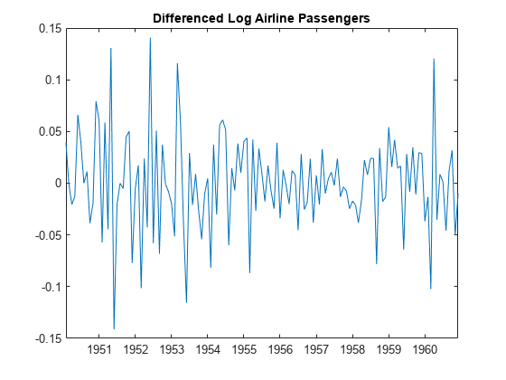
Calculate the differenced series, $$(1-L)(1-L^{12})y_t$$, where $$y_t$$ is the original log-transformed data. Plot the differenced series.

A1 = LagOp({1,-1},Lags=[0 1]);
A12 = LagOp({1,-1},Lags=[0 12]);
dY = filter(A1*A12,y);
dT = T - length(dY);

figure
plot(DataTimeTable.Time((dT+1):T),dY)
title("Differenced Log Airline Passengers")

The differenced series appears stationary.

Plot the sample autocorrelation function (ACF).

figure
autocorr(dY,NumLags=50)

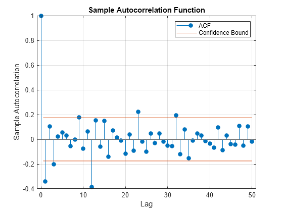
The sample ACF of the differenced series shows significant autocorrelation at lags that are multiples of 12. There is also potentially significant autocorrelation at smaller lags.

Specify a seasonal ARIMA model.

Box, Jenkins, and Reinsel suggest the multiplicative seasonal model,

for this data set [1].

Specify this model.

Mdl = arima(Constant=0,D=1,Seasonality=12, ...
    MALags=1,SMALags=12)

Mdl = 
  arima with properties:

     Description: "ARIMA(0,1,1) Model Seasonally Integrated with Seasonal MA(12) (Gaussian Distribution)"
      SeriesName: "Y"
    Distribution: Name = "Gaussian"
               P: 13
               D: 1
               Q: 13
        Constant: 0
              AR: {}
             SAR: {}
              MA: {NaN} at lag [1]
             SMA: {NaN} at lag [12]
     Seasonality: 12
            Beta: [1×0]
        Variance: NaN

The property P is equal to 13, corresponding to the sum of the nonseasonal and seasonal differencing degrees (1 + 12). The property Q is also equal to 13, corresponding to the sum of the degrees of the nonseasonal and seasonal MA polynomials (1 + 12). Parameters that need to be estimated have value NaN.