Create Seasonal ARIMA (SARIMA) Models

These examples show how to create various multiplicative seasonal autoregressive integrated moving average (SARIMA) models by using the arima function. For an overview on conditional mean model creation, see Represent Univariate Dynamic Conditional Mean Models in MATLAB.

Seasonal ARIMA Model with No Constant Term

Open Live Script

This example shows how to use arima to specify a SARIMA model (for monthly data) with no constant term.

Specify a SARIMA model with no constant term,

$(1 - ϕ_{1} L) (1 - Φ_{12} L^{12}) (1 - L)^{1} (1 - L^{12}) y_{t} = (1 + θ_{1} L) (1 + Θ_{12} L^{12}) ε_{t},$

where the innovation distribution is Gaussian with constant variance. Here, $(1 - L)^{1}$ is the first degree nonseasonal differencing operator and $(1 - L^{12})$ is the first degree seasonal differencing operator with periodicity 12.

Mdl = arima('Constant',0,'ARLags',1,'SARLags',12,'D',1,...
            'Seasonality',12,'MALags',1,'SMALags',12)

Mdl = 
  arima with properties:

     Description: "ARIMA(1,1,1) Model Seasonally Integrated with Seasonal AR(12) and MA(12) (Gaussian Distribution)"
      SeriesName: "Y"
    Distribution: Name = "Gaussian"
               P: 26
               D: 1
               Q: 13
        Constant: 0
              AR: {NaN} at lag [1]
             SAR: {NaN} at lag [12]
              MA: {NaN} at lag [1]
             SMA: {NaN} at lag [12]
     Seasonality: 12
            Beta: [1×0]
        Variance: NaN

The name-value pair argument ARLags specifies the lag corresponding to the nonseasonal AR coefficient, $ϕ_{1}$ . SARLags specifies the lag corresponding to the seasonal AR coefficient, here at lag 12. The nonseasonal and seasonal MA coefficients are specified similarly. D specifies the degree of nonseasonal integration. Seasonality specifies the periodicity of the time series, for example Seasonality = 12 indicates monthly data. Since Seasonality is greater than 0, the degree of seasonal integration $D_{s}$ is one.

Whenever you include seasonal AR or MA polynomials (signaled by specifying SAR or SMA) in the model specification, arima incorporates them as factors in the model (multiplicative seasonal ARIMA). arima sets the property P equal to p + D + $p_{s}$ + s (here, 1 + 1 + 12 + 12 = 26). Similarly, arima sets the property Q equal to q + $q_{s}$ (here, 1 + 12 = 13).

Display the value of SAR:

Mdl.SAR

ans=1×12 cell array
    {[0]}    {[0]}    {[0]}    {[0]}    {[0]}    {[0]}    {[0]}    {[0]}    {[0]}    {[0]}    {[0]}    {[NaN]}

The SAR cell array returns 12 elements, as specified by SARLags. arima sets the coefficients at interim lags equal to zero to maintain consistency with MATLAB® cell array indexing. Therefore, the only nonzero coefficient corresponds to lag 12.

All of the other properties of Mdl are NaN-valued, indicating that the corresponding model parameters are estimable, or you can specify their value by using dot notation.

Seasonal ARIMA Model with Known Parameter Values

Open Live Script

This example shows how to specify a SARIMA model (for quarterly data) with known parameter values. You can use such a fully specified model as an input to simulate or forecast.

Specify the SARIMA model

$(1 - . 5 L) (1 + 0.7 L^{4}) (1 - L)^{1} (1 - L^{4}) y_{t} = (1 + . 3 L) (1 - . 2 L^{4}) ε_{t},$

where the innovation distribution is Gaussian with constant variance 0.15. Here, $(1 - L)^{1}$ is the nonseasonal differencing operator and $(1 - L^{4})$ is the first degree seasonal differencing operator with periodicity 4.

Mdl = arima('Constant',0,'AR',0.5,'D',1,'MA',0.3,...
    'Seasonality',4,'SAR',-0.7,'SARLags',4,...
    'SMA',-0.2,'SMALags',4,'Variance',0.15)

Mdl = 
  arima with properties:

     Description: "ARIMA(1,1,1) Model Seasonally Integrated with Seasonal AR(4) and MA(4) (Gaussian Distribution)"
      SeriesName: "Y"
    Distribution: Name = "Gaussian"
               P: 10
               D: 1
               Q: 5
        Constant: 0
              AR: {0.5} at lag [1]
             SAR: {-0.7} at lag [4]
              MA: {0.3} at lag [1]
             SMA: {-0.2} at lag [4]
     Seasonality: 4
            Beta: [1×0]
        Variance: 0.15

The output specifies the nonseasonal and seasonal AR coefficients with opposite signs compared to the lag polynomials. This is consistent with the difference equation form of the model. The output specifies the lags of the seasonal AR and MA coefficients using SARLags and SMALags, respectively. D specifies the degree of nonseasonal integration. Seasonality = 4 specifies quarterly data with one degree of seasonal integration.

All parameter values are specified, that is, no object property is NaN-valued.

Specify Seasonal ARIMA (SARIMA) Model Using Econometric Modeler App

In the Econometric Modeler app, you can specify the lag structure, presence of a constant, and innovation distribution of a SARIMA(p,D,q)×(p_s,D_s,q_s)_s model by following these steps. All specified coefficients are unknown but estimable parameters.

At the command line, open the Econometric Modeler app.
```
econometricModeler
```
Alternatively, open the app from the apps gallery (see Econometric Modeler).
In the Time Series pane, select the response time series to which the model will be fit.
On the Modeler tab, in the Models section, click the arrow to display the models gallery.
In the ARIMA Models section of the gallery, click SARIMA. To create SARIMAX models, see Create ARIMA Models That Include Exogenous Covariates.
The SARIMA Model Parameters dialog box appears.
Specify the lag structure. Use the Lag Order tab to specify a SARIMA(p,D,q)×(p_s,D_s,q_s)_s model that includes:
- All consecutive lags from 1 through their respective orders, in the nonseasonal polynomials
- Lags that are all consecutive multiples of the period (s), in the seasonal polynomials
- An s-degree seasonal integration polynomial
Use the Lag Vector tab for the flexibility to specify particular lags for all polynomials. For more details, see Specifying Univariate Lag Operator Polynomials Interactively. Regardless of the tab you use, you can verify the model form by inspecting the equation in the Model Equation section.

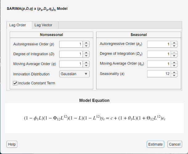
For example, consider this SARIMA(2,1,1)×(2,1,1)₁₂ model.

$(1 - ϕ_{1} L - ϕ_{2} L^{2}) (1 - Φ_{12} L^{12} - Φ_{24} L^{24}) (1 - L) (1 - L^{12}) y_{t} = c + (1 + θ_{1} L) (1 + Θ_{12} L^{12}) ε_{t},$

where ε_t is a series of IID Gaussian innovations.

The model includes all consecutive AR and MA lags from 1 through their respective orders. Also, the lags of the SAR and SMA polynomials are consecutive multiples of the period from 12 through their respective specified order times 12. Therefore, use the Lag Order tab to specify the model.

In the Nonseasonal section:
1. Set Degree of Integration (p) to 1.
2. Set Autoregressive Order (D) to 2.
3. Set Moving Average Order (q) to 1.
In the Seasonal section:
1. Set Seasonality to 12.
2. Set Autoregressive Order (p_s) to 2. This input specifies the inclusion of SAR lags 12 and 24 (that is, the first and second multiples of the value of Seasonality).
3. Set Degree of Integration (D_s) to 1. This input specifies the inclusion of a seasonal difference term (1 – L^s), where s is Seasonality. Econometric Modeler supports zero or one degrees of seasonal differencing.
4. Set Moving Average Order to 1. This input specifies the inclusion of SMA lag 12 (that is, the first multiple of the value of Seasonality).
5. Select the check box.
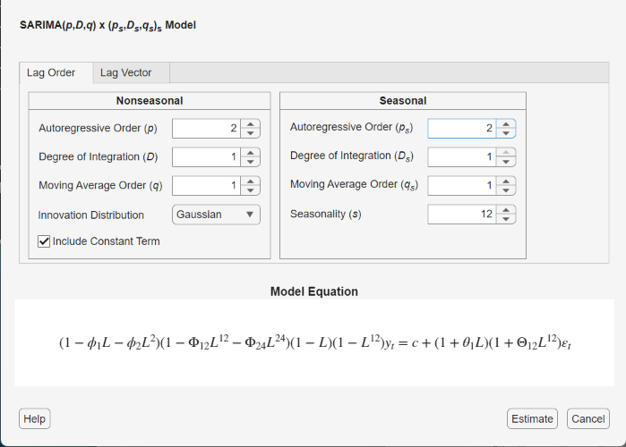
Verify that the equation in the Model Equation section matches your model.

To exclude a constant from the model and to specify that the innovations are Gaussian, follow the previous steps, and clear the Include Constant Term check box.
To specify t-distributed innovations, follow the previous steps, and click the Innovation Distribution button, then select t.

For another example, consider this SARIMA(12,1,1)×(2,1,1)₁₂ model.

$(1 - ϕ_{1} L - ϕ_{12} L^{12}) (1 - Φ_{24} L^{24}) (1 - L) (1 - L^{12}) y_{t} = c + (1 + θ_{1} L) (1 + Θ_{12} L^{12}) ε_{t} .$

The model does not include consecutive AR lags, and the lags of the SAR polynomial are not consecutive multiples of the period. Therefore, use the Lag Vector tab to specify this model:

In the SARIMA Model Parameters dialog box, click the Lag Vector tab.
In the Nonseasonal section:
1. Set Degree of Integration to 1.
2. Set Autoregressive Lags to 1 12.
3. Set Moving Average Lags to 1.
In the Seasonal section:
1. Set Seasonality to 12. The app includes a 12-degree seasonal integration polynomial.
2. Set Autoregressive Lags to 24. This input specifies the inclusion of SAR lag 24. The input is independent of the value in the Seasonality box.
3. Set Moving Average Lags to 12. This input specifies the inclusion of SMA lag 12. The input is independent of the value in the Seasonality box.
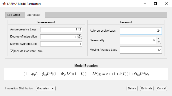
Verify that the equation in the Model Equation section matches your model.

After you specify a model, click Estimate to estimate all unknown parameters in the model.

What Are Seasonal ARIMA (SARIMA) Models?

Time series collected periodically, such as quarterly or monthly, can exhibit a seasonal trend, a relationship between observations made during the same period in successive years. In addition to this seasonal relationship, a relationship between observations during successive periods might exist. The multiplicative seasonal ARIMA (SARIMA) model is an extension of the ARIMA model that addresses seasonality and potential seasonal unit roots [1].

For a series with periodicity s, the SARIMA(p,D,q)×(p_s,D_s,q_s)_s in lag operator polynomial notation is

$ϕ (L) Φ (L) {(1 - L)}^{D} {(1 - L^{s})}^{D_{s}} y_{t} = c + θ (L) Θ (L) ε_{t} .$

This list briefly describes the components in the equation; for details on the connections between the parameters and software, see ARIMA Model Parameters and Corresponding Object Properties.

$ϕ (L) = (1 - ϕ_{1} L - \dots - ϕ_{p} L^{p})$ is the degree p stable, nonseasonal AR lag operator polynomial.
(1 – L)^D is the order D nonseasonal backward difference polynomial; it accounts for nonstationarity in observations made in successive periods.
$θ (L) = (1 + θ_{1} L + \dots + θ_{q} L^{q})$ is the degree q invertible, nonseasonal MA lag operator polynomial.
$Φ (L) = 1 - Φ_{p_{1}} L^{p_{1}} - Φ_{p_{2}} L^{p_{2}} - ... - Φ_{p_{s}} L^{p_{s}}$ is the degree p_s stable, seasonal AR lag polynomial.
$Θ (L) = 1 + Θ_{q_{1}} L^{q_{1}} + Θ_{q_{2}} L^{q_{2}} + ... + Θ_{q_{s}} L^{q_{s}}$ is the degree q_s invertible, seasonal MA lag operator polynomial.
(1 – L^s)^D_s is the order D_s seasonal backward difference polynomial; it accounts for nonstationarity in observations made in the same period in successive years. When you specify s ≥ 0 (Seasonailty), Econometrics Toolbox™ sets D_s to 1. D_s is 0 otherwise.
ε_t is an uncorrelated innovation process with mean zero.

Tip

When you create a SARIMA model, set the lags associated with the seasonal polynomials in the periodicity of the observed data (e.g., 4, 8,... for quarterly data, or 12, 24,... for monthly data), and not as multiples of the seasonality (e.g., 1, 2,...). This convention does not conform to standard Box and Jenkins notation, but is a more flexible approach for incorporating multiplicative seasonality.

References

[1] Box, George E. P., Gwilym M. Jenkins, and Gregory C. Reinsel. Time Series Analysis: Forecasting and Control. 3rd ed. Englewood Cliffs, NJ: Prentice Hall, 1994.

Create Seasonal ARIMA (SARIMA) Models

Seasonal ARIMA Model with No Constant Term

Seasonal ARIMA Model with Known Parameter Values

Specify Seasonal ARIMA (SARIMA) Model Using Econometric Modeler App

What Are Seasonal ARIMA (SARIMA) Models?

References

See Also

Apps

Objects

Functions

Topics