Bayesian Lasso Regression
This example shows how to perform variable selection by using Bayesian lasso regression.
Lasso regression is a linear regression technique that combines regularization and variable selection. Regularization helps prevent overfitting by decreasing the magnitude of the regression coefficients. The frequentist view of lasso regression differs from that of other regularization techniques, such as, ridge regression, because lasso attributes a value of exactly 0 to regression coefficients corresponding to predictors that are insignificant or redundant.
Consider this multiple linear regression model:
is a vector of n responses.
is a matrix of p corresponding observed predictor variables.
is a vector of p regression coefficients.
is the intercept.
is a length n column vector of ones.
is a random vector of iid Gaussian disturbances with a mean of 0 and variance of .
The objective function of the frequentist view of lasso regression is
is the penalty (or shrinkage) term and, unlike other parameters, is not fit to the data. You must specify a value for before estimation, and a best practice is to tune it. After you specify a value, is minimized with respect to the regression coefficients. The resulting coefficients are the lasso estimates. For more details on the frequentist view of lasso regression, see [1].
For this example, consider creating a predictive linear model for the US unemployment rate. You want a model that generalizes well. In other words, you want to minimize the model complexity by removing all redundant predictors and all predictors that are uncorrelated with the unemployment rate.
Load and Preprocess Data
Load the US macroeconomic data set Data_USEconModel.mat.
load Data_USEconModelThe data set includes the MATLAB® timetable DataTimeTable, which contains 14 variables measured from Q1 1947 through Q1 2009; UNRATE is the US unemployment rate. For more details, enter Description at the command line.
Plot all series in the same figure, but in separate subplots.
figure
tiledlayout(4,4)
for j = 1:size(DataTimeTable,2)
    nexttile
    plot(DataTimeTable.Time,DataTimeTable{:,j});
    title(DataTimeTable.Properties.VariableNames(j));
end
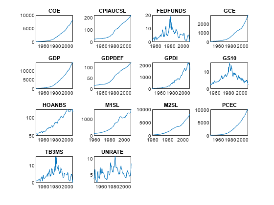
All series except FEDFUNDS, GS10, TB3MS, and UNRATE appear to have an exponential trend.
Apply the log transform to those variables that have an exponential trend.
hasexpotrend = ~ismember(DataTimeTable.Properties.VariableNames,...
    ["FEDFUNDS" "GD10" "TB3MS" "UNRATE"]);
DataTimeTableLog = varfun(@log,DataTimeTable, ...
    InputVariables=DataTimeTable.Properties.VariableNames(hasexpotrend));
DataTimeTableLog = [DataTimeTableLog DataTimeTable(:,DataTimeTable.Properties.VariableNames(~hasexpotrend))];
DataTimeTableLog is a timetable like DataTimeTable, but those variables with an exponential trend are on the log scale.
Coefficients that have relatively large magnitudes tend to dominate the penalty in the lasso regression objective function. Therefore, it is important that variables have a similar scale when you implement lasso regression. Compare the scales of the variables in DataTimeTableLog by plotting their box plots on the same axis.
figure
boxplot(DataTimeTableLog.Variables,Labels=DataTimeTableLog.Properties.VariableNames);
h = gca;
h.XTickLabelRotation = 45;
title("Variable Box Plots");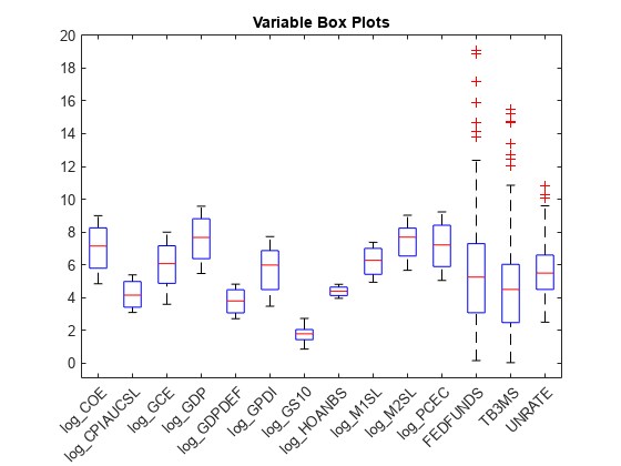
The variables have fairly similar scales.
To determine how well time series models generalize, follow this procedure:
Partition the data into estimation and forecast samples.
Fit the models to the estimation sample.
Use the fitted models to forecast responses into the forecast horizon.
Estimate the forecast mean squared error (FMSE) for each model.
Choose the model with the lowest FMSE.
Create estimation and forecast sample variables for the response and predictor data. Specify a forecast horizon of 4 years (16 quarters).
fh = 16;
y = DataTimeTableLog.UNRATE(1:(end - fh));
yF = DataTimeTableLog.UNRATE((end - fh + 1):end);
isresponse = DataTimeTable.Properties.VariableNames == "UNRATE";
X = DataTimeTableLog{1:(end - fh),~isresponse};
XF = DataTimeTableLog{(end - fh + 1):end,~isresponse};
p = size(X,2); % Number of predictors
predictornames = DataTimeTableLog.Properties.VariableNames(~isresponse);
Fit Simple Linear Regression Model
Fit a simple linear regression model to the estimation sample. Specify the variable names (the name of the response variable must be the last element). Extract the p-values. Identify the insignificant coefficients by using a 5% level of significance.
SLRMdlFull = fitlm(X,y,VarNames=DataTimeTableLog.Properties.VariableNames)
SLRMdlFull =
Linear regression model:
    UNRATE ~ 1 + log_COE + log_CPIAUCSL + log_GCE + log_GDP + log_GDPDEF + log_GPDI + log_GS10 + log_HOANBS + log_M1SL + log_M2SL + log_PCEC + FEDFUNDS + TB3MS

Estimated Coefficients:
                    Estimate       SE        tStat       pValue
                    ________    ________    _______    __________

    (Intercept)       88.014      5.3229     16.535    2.6568e-37
    log_COE           7.1111      2.3426     3.0356     0.0027764
    log_CPIAUCSL     -3.4032      2.4611    -1.3828       0.16853
    log_GCE            -5.63      1.1581    -4.8615    2.6245e-06
    log_GDP           14.522      3.9406     3.6851    0.00030659
    log_GDPDEF        11.926      2.9298     4.0704    7.1598e-05
    log_GPDI         -2.5939     0.54603    -4.7504    4.2792e-06
    log_GS10         0.57467     0.29313     1.9605      0.051565
    log_HOANBS       -32.861      1.4507    -22.652    2.3116e-53
    log_M1SL         -3.3023     0.53185     -6.209     3.914e-09
    log_M2SL         -1.3845      1.0438    -1.3264       0.18647
    log_PCEC          -7.143      3.4302    -2.0824      0.038799
    FEDFUNDS        0.044542    0.047747    0.93287        0.3522
    TB3MS            -0.1577    0.064421     -2.448      0.015375


Number of observations: 185, Error degrees of freedom: 171
Root Mean Squared Error: 0.312
R-squared: 0.957,  Adjusted R-Squared: 0.954
F-statistic vs. constant model: 292, p-value = 2.26e-109
slrPValue = SLRMdlFull.Coefficients.pValue;
isInSig = SLRMdlFull.CoefficientNames(slrPValue > 0.05)
isInSig = 1×4 cell
    {'log_CPIAUCSL'}    {'log_GS10'}    {'log_M2SL'}    {'FEDFUNDS'}
SLRMdlFull is a LinearModel model object. The p-values suggest that, at a 5% level of significance, CPIAUCSL, GS10, M2SL, and FEDFUNDS are insignificant variables.
Refit the linear model without the insignificant variables in the predictor data. Using the full and reduced models, predict the unemployment rate into the forecast horizon, then estimate the FMSEs.
idxreduced = ~ismember(predictornames,isInSig);
XReduced = X(:,idxreduced);
SLRMdlReduced = fitlm(XReduced,y, ...
    VarNames=[predictornames(idxreduced) {'UNRATE'}]);

yFSLRF = predict(SLRMdlFull,XF);
yFSLRR = predict(SLRMdlReduced,XF(:,idxreduced));

fmseSLRF = sqrt(mean((yF - yFSLRF).^2))
fmseSLRF =
0.6674
fmseSLRR = sqrt(mean((yF - yFSLRR).^2))
fmseSLRR =
0.6105
The FMSE of the reduced model is less than the FMSE of the full model, which suggests that the reduced model generalizes better.
Fit Frequentist Lasso Regression Model
Fit a lasso regression model to the data. Use the default regularization path. lasso standardizes the data by default. Because the variables are on similar scales, do not standardize them. Return information about the fits along the regularization path.
[LassoBetaEstimates,FitInfo] = lasso(X,y,Standardize=false, ...
    PredictorNames=predictornames);
By default, lasso fits the lasso regression model 100 times by using a sequence of values for . Therefore, LassoBetaEstimates is a 13-by-100 matrix of regression coefficient estimates. Rows correspond to predictor variables in X, and columns correspond to values of . FitInfo is a structure that includes the values of (FitInfo.Lambda), the mean squared error for each fit (FitInfo.MSE), and the estimated intercepts (FitInfo.Intercept).
Compute the FMSE of each model returned by lasso.
yFLasso = FitInfo.Intercept + XF*LassoBetaEstimates;
fmseLasso = sqrt(mean((yF - yFLasso).^2,1));
Plot the magnitude of the regression coefficients with respect to the shrinkage value.
hax = lassoPlot(LassoBetaEstimates,FitInfo);
L1Vals = hax.Children.XData;
yyaxis right
h = plot(L1Vals,fmseLasso,LineWidth=2,LineStyle="--");
legend(h,"FMSE",Location="southwest");
ylabel("FMSE");
title("Frequentist Lasso")
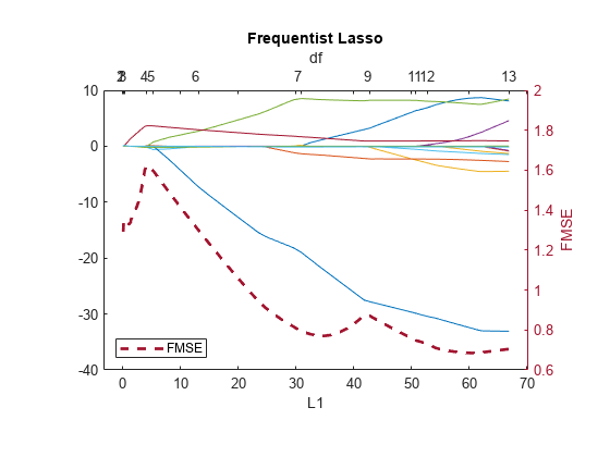
A model with 7 predictors (df = 7) seems to balance minimal FMSE and model complexity well. Obtain the coefficients corresponding to the model containing 7 predictors and yielding minimal FMSE.
fmsebestlasso = min(fmseLasso(FitInfo.DF == 7));
idx = fmseLasso == fmsebestlasso;
bestLasso = [FitInfo.Intercept(idx); LassoBetaEstimates(:,idx)];
table(bestLasso,RowNames=["Intercept" predictornames])ans=14×1 table
bestLasso
_________
Intercept 61.154
log_COE 0.042061
log_CPIAUCSL 0
log_GCE 0
log_GDP 0
log_GDPDEF 8.524
log_GPDI 0
log_GS10 1.6957
log_HOANBS -18.937
log_M1SL -1.3365
log_M2SL 0.17948
log_PCEC 0
FEDFUNDS 0
TB3MS -0.14459
The frequentist lasso analysis suggests that the variables CPIAUCSL, GCE, GDP, GPDI, PCEC, and FEDFUNDS are either insignificant or redundant.
Fit Bayesian Lasso Regression Model
In the Bayesian view of lasso regression, the prior distribution of the regression coefficients is Laplace (double exponential), with mean 0 and scale , where is the fixed shrinkage parameter and . For more details, see lassoblm.
As with the frequentist view of lasso regression, if you increase , then the sparsity of the resulting model increases monotonically. However, unlike frequentist lasso, Bayesian lasso has insignificant or redundant coefficient modes that are not exactly 0. Instead, estimates have a posterior distribution and are insignificant or redundant if the region around 0 has high density.
When you implement Bayesian lasso regression in MATLAB®, be aware of several differences between the Statistics and Machine Learning Toolbox™ function lasso and the Econometrics Toolbox™ object lassoblm and its associated functions.
lassoblmis part of an object framework, whereaslassois a function. The object framework streamlines econometric workflows.Unlike
lasso,lassoblmdoes not standardize the predictor data. However, you can supply different shrinkage values for each coefficient. This feature helps maintain the interpretability of the coefficient estimates.lassoblmapplies one shrinkage value to each coefficient; it does not accept a regularization path likelasso.
Because the lassoblm framework is suited to performing Bayesian lasso regression for one shrinkage value per coefficient, you can use a for loop to perform lasso over a regularization path.
Create a Bayesian lasso regression prior model by using bayeslm. Specify the number of predictor variables and the variable names. Display the default shrinkage value for each coefficient stored in the Lambda property of the model.
PriorMdl = bayeslm(p,ModelType="lasso",VarNames=predictornames);
table(PriorMdl.Lambda,RowNames=PriorMdl.VarNames)ans=14×1 table
Var1
____
Intercept 0.01
log_COE 1
log_CPIAUCSL 1
log_GCE 1
log_GDP 1
log_GDPDEF 1
log_GPDI 1
log_GS10 1
log_HOANBS 1
log_M1SL 1
log_M2SL 1
log_PCEC 1
FEDFUNDS 1
TB3MS 1
PriorMdl is a lassoblm model object. lassoblm attributes a shrinkage of 1 for each coefficient except the intercept, which has a shrinkage of 0.01. These default values might not be useful in most applications; a best practice is to experiment with many values.
Consider the regularization path returned by lasso. Inflate the shrinkage values by a factor of , where is the MSE of lasso run , = 1 through the number of shrinkage values.
ismissing = any(isnan(X),2);
n = sum(~ismissing); % Effective sample size
lambda = FitInfo.Lambda*n./sqrt(FitInfo.MSE);
Consider the regularization path returned by lasso. Loop through the shrinkage values at each iteration:
Estimate the posterior distributions of the regression coefficients and the disturbance variance, given the shrinkage and data. Because the scales of the predictors are close, attribute the same shrinkage to each predictor, and attribute a shrinkage of
0.01to the intercept. Store the posterior means and 95% credible intervals.For the lasso plot, if a 95% credible interval includes 0, then set the corresponding posterior mean to zero.
Forecast into the forecast horizon.
Estimate the FMSE.
numlambda = numel(lambda);

% Preallocate
BayesLassoCoefficients = zeros(p+1,numlambda);
BayesLassoCI95 = zeros(p+1,2,numlambda);
fmseBayesLasso = zeros(numlambda,1);
BLCPlot = zeros(p+1,numlambda);

% Estimate and forecast
rng(10); % For reproducibility
for j = 1:numlambda
    PriorMdl.Lambda = lambda(j);
    [EstMdl,Summary] = estimate(PriorMdl,X,y,Display=false);
    BayesLassoCoefficients(:,j) = Summary.Mean(1:(end - 1));
    BLCPlot(:,j) = Summary.Mean(1:(end - 1));
    BayesLassoCI95(:,:,j) = Summary.CI95(1:(end - 1),:);
    idx = BayesLassoCI95(:,2,j) > 0 & BayesLassoCI95(:,1,j) <= 0;
    BLCPlot(idx,j) = 0;
    yFBayesLasso = forecast(EstMdl,XF);
    fmseBayesLasso(j) = sqrt(mean((yF - yFBayesLasso).^2));
end
At each iteration, estimate runs a Gibbs sampler to sample from the full conditionals (see Analytically Tractable Posteriors) and returns the empiricalblm model EstMdl, which contains the draws and the estimation summary table Summary. You can specify parameters for the Gibbs sampler, such as the number of draws or thinning scheme.
A good practice is to diagnose the posterior sample by inspecting trace plots. However, because 100 distributions were drawn, this example proceeds without performing that step.
Plot the posterior means of the coefficients with respect to the normalized L1 penalties (sum of the magnitudes of the coefficients except the intercept). On the same plot, but in the right y axis, plot the FMSEs.
L1Vals = sum(abs(BLCPlot(2:end,:)),1)/max(sum(abs(BLCPlot(2:end,:)),1));

figure;
plot(L1Vals,BLCPlot(2:end,:))
xlabel("L1");
ylabel("Coefficient Estimates");
yyaxis right
h = plot(L1Vals,fmseBayesLasso,LineWidth=2,LineStyle="--");
legend(h,"FMSE",Location="southwest");
ylabel("FMSE");
title("Bayesian Lasso")
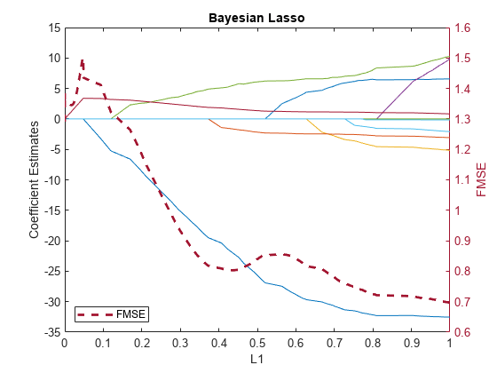
The model tends to generalize better as the normalized L1 penalty increases past 0.1. To balance minimal FMSE and model complexity, choose the simplest model with FMSE closest to 0.68.
idx = find(fmseBayesLasso > 0.68,1);
fmsebestbayeslasso = fmseBayesLasso(idx);
bestBayesLasso = BayesLassoCoefficients(:,idx);
bestCI95 = BayesLassoCI95(:,:,idx);
table(bestBayesLasso,bestCI95,RowNames=["Intercept" predictornames])ans=14×2 table
bestBayesLasso bestCI95
______________ ______________________
Intercept 90.587 79.819 101.62
log_COE 6.5591 1.8093 11.239
log_CPIAUCSL -2.2971 -6.9019 1.7057
log_GCE -5.1707 -7.4902 -2.8583
log_GDP 9.8839 2.3848 17.672
log_GDPDEF 10.281 5.1677 15.936
log_GPDI -2.0973 -3.2168 -0.96728
log_GS10 0.82485 0.22748 1.4237
log_HOANBS -32.538 -35.589 -29.526
log_M1SL -3.0656 -4.1499 -2.0066
log_M2SL -1.1007 -3.1243 0.75844
log_PCEC -3.3342 -9.6496 1.8482
FEDFUNDS 0.043672 -0.056192 0.14254
TB3MS -0.15682 -0.29385 -0.022145
One way to determine if a variable is insignificant or redundant is by checking whether 0 is in its corresponding coefficient 95% credible interval. Using this criterion, CPIAUCSL, M2SL, PCEC, and FEDFUNDS are insignificant.
Display all estimates in a table for comparison.
SLRR = zeros(p + 1,1);
SLRR([true idxreduced]) = SLRMdlReduced.Coefficients.Estimate;
table([SLRMdlFull.Coefficients.Estimate; fmseSLRR], ...
    [SLRR; fmseSLRR],[bestLasso; fmsebestlasso], ...
    [bestBayesLasso; fmsebestbayeslasso], ...
    VariableNames=["SLRFull" "SLRReduced" "Lasso" "BayesLasso"], ...
    RowNames=[PriorMdl.VarNames; "MSE"])
ans=15×4 table
                    SLRFull     SLRReduced     Lasso      BayesLasso
                    ________    __________    ________    __________

    Intercept         88.014       88.327       61.154       90.587
    log_COE           7.1111       10.854     0.042061       6.5591
    log_CPIAUCSL     -3.4032            0            0      -2.2971
    log_GCE            -5.63      -6.1958            0      -5.1707
    log_GDP           14.522       16.701            0       9.8839
    log_GDPDEF        11.926       9.1106        8.524       10.281
    log_GPDI         -2.5939      -2.6963            0      -2.0973
    log_GS10         0.57467            0       1.6957      0.82485
    log_HOANBS       -32.861      -33.782      -18.937      -32.538
    log_M1SL         -3.3023      -2.8099      -1.3365      -3.0656
    log_M2SL         -1.3845            0      0.17948      -1.1007
    log_PCEC          -7.143      -14.207            0      -3.3342
    FEDFUNDS        0.044542            0            0     0.043672
    TB3MS            -0.1577    -0.078449     -0.14459     -0.15682
    MSE              0.61048      0.61048      0.79425      0.69639
After you chose a model, re-estimate it using the entire data set. For example, to create a predictive Bayesian lasso regression model, create a prior model and specify the shrinkage yielding the simplest model with the minimal FMSE, then estimate it using the entire data set.
bestLambda = lambda(idx);
PriorMdl = bayeslm(p,ModelType="lasso",Lambda=bestLambda, ...
    VarNames=predictornames);
PosteriorMdl = estimate(PriorMdl,[X; XF],[y; yF]);
Method: lasso MCMC sampling with 10000 draws
Number of observations: 201
Number of predictors:   14

              |   Mean      Std          CI95         Positive  Distribution
-----------------------------------------------------------------------------
 Intercept    |  85.9694  5.2085   [75.704, 96.205]     1.000     Empirical
 log_COE      |  12.3830  2.1464   [ 8.141, 16.605]     1.000     Empirical
 log_CPIAUCSL |   0.1730  1.9162   [-3.598,  4.096]     0.531     Empirical
 log_GCE      |  -7.1946  1.0625   [-9.271, -5.109]     0.000     Empirical
 log_GDP      |  11.7841  3.9844   [ 4.050, 19.632]     0.999     Empirical
 log_GDPDEF   |   8.8783  2.4254   [ 3.907, 13.643]     1.000     Empirical
 log_GPDI     |  -2.5830  0.5319   [-3.618, -1.547]     0.000     Empirical
 log_GS10     |   0.6896  0.2563   [ 0.202,  1.195]     0.996     Empirical
 log_HOANBS   | -32.3169  1.4870  [-35.260, -29.381]    0.000     Empirical
 log_M1SL     |  -2.2348  0.5017   [-3.223, -1.259]     0.000     Empirical
 log_M2SL     |   0.3780  0.9101   [-1.384,  2.194]     0.659     Empirical
 log_PCEC     | -11.2734  3.0197  [-17.208, -5.239]     0.000     Empirical
 FEDFUNDS     |  -0.0134  0.0483   [-0.109,  0.080]     0.393     Empirical
 TB3MS        |  -0.1127  0.0652   [-0.239,  0.015]     0.044     Empirical
 Sigma2       |   0.1186  0.0123   [ 0.097,  0.145]     1.000     Empirical
References
See Also
estimate | simulate | forecast