Mean-Variance Portfolio Optimization with Entropy Pooling

Baseline Mean-Variance Optimization

A common objective in mean-variance portfolio optimization is to maximize the Sharpe ratio, which is the ratio of expected return to volatility. Load the dowPortfolio.xlsx data set, which includes daily price data for 30 assets and one benchmark. Select seven assets to form the investment universe.

T = readtable("dowPortfolio.xlsx");
assetNames = ["AA" "AIG" "WMT" "MSFT" "BA" "GE" "IBM"];
assetReturns = tick2ret(T(:,assetNames));
numAssets = width(assetReturns);

Use the Portfolio object to find the maximum Sharpe ratio portfolio under a fully invested, long-only constraint. First, compute the sample mean and covariance using the estimateAssetMoments function. Then, solve for the portfolio weights using the estimateMaxSharpeRatio function.

port = Portfolio(NumAssets=numAssets,lb=0,budget=1,Name="Mean Variance");
port = estimateAssetMoments(port,assetReturns);
weightsBaseline = estimateMaxSharpeRatio(port);
disp(weightsBaseline)

    0.0000
    0.0000
    0.0000
    0.0594
    0.3207
    0.0000
    0.6199

The entries in weightsBaseline are the respective fractions of investment dedicated to each asset in the portfolio. These fractions maximize the Sharpe ratio, given the historical returns and the selected investment universe, and serve as the baseline allocation before you incorporate any views.

Update Distribution with Entropy Pooling

The baseline optimization relies entirely on historical data. However, in practice, an investor might have forward-looking views about certain assets that differ from the historical data. Entropy pooling provides a way to incorporate such views into the empirical distribution of returns.

Treat the historical returns as a set of $$J$$ equally likely scenarios. The entropy pooling algorithm then finds new probability weights $$p=\left(p_1,p_2,\dots ,p_J\right)$$ for these scenarios such that the weighted distribution satisfies the investor's view constraints, while staying as close as possible to the original uniform weights, as measured by relative entropy (Kullback–Leibler divergence).

To create and solve this type of problem, you use the entropyViews object. This example specifies four views, all with annualized targets: the first two are absolute mean views, the third is a relative mean view, and the fourth is a volatility view.

Because AIG has both a mean view and a volatility view, use the sequential entropy pooling approach [2]. First, solve using only the mean views. Then, use the posterior as the prior in a second solve that adds the volatility view. This two-step procedure corrects the second-moment target so that the volatility view is satisfied exactly. For a detailed explanation of the sequential entropy pooling approach, see Incorporate Nonlinear View Constraints Using Sequential Entropy Pooling.

Create an entropyViews object and impose the mean views. Convert the annualized targets to daily returns to match the scenario data. To express the view that MSFT outperforms IBM, augment the scenario matrix with a derived column representing the return difference.

bizyear2bizday = 1/252;
augmentedReturns = assetReturns;
augmentedReturns.MSFT_minus_IBM = augmentedReturns.MSFT-augmentedReturns.IBM;

evMean = entropyViews(augmentedReturns);
evMean = setMeanViews(evMean,["AIG" "WMT" "MSFT_minus_IBM"],"=",[0.05 0.03 0.05]*bizyear2bizday);

Solve for the posterior weights using only the mean views.

pMean = posteriorProbabilities(evMean);

Now perform the sequential step. Use the posterior weights in pMean as the prior weights, and include the volatility view on AIG with the mean views.

pMean = pMean/sum(pMean);
evSeq = entropyViews(augmentedReturns,PriorProbabilities=pMean);
evSeq = setMeanViews(evSeq,["AIG" "WMT" "MSFT_minus_IBM"],"=",[0.05 0.03 0.05]*bizyear2bizday);
evSeq = setVolatilityViews(evSeq,"AIG","=",0.2*sqrt(bizyear2bizday));

Solve for the final posterior weights.

p = posteriorProbabilities(evSeq);

Optimize Portfolio Using Updated Distribution

Compute the updated mean and covariance of asset returns using the posterior probability weights p. These weights replace the historical moments in the portfolio optimization.

portfolioEP = Portfolio(NumAssets=numAssets,lb=0,budget=1,Name="Mean Variance with Entropy Pooling");
portfolioEP = estimateAssetMoments(portfolioEP,assetReturns,Probabilities=p);

Find the new maximum Sharpe ratio portfolio.

weightsEP = estimateMaxSharpeRatio(portfolioEP);

Compare Baseline and Adjusted Allocations

Compare the portfolio allocations before and after incorporating the investor views.

figure;
tiledlayout(1,2);
idx = weightsBaseline > 0.001;
nexttile
pie(weightsBaseline(idx),assetNames(idx))
title(port.Name)

idxEP = weightsEP > 0.001;
nexttile
pie(weightsEP(idxEP), assetNames(idxEP))
title(portfolioEP.Name)

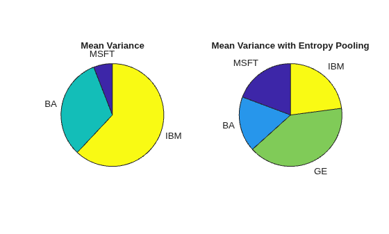
Display the allocations side-by-side in a table.

disp(table(assetNames',weightsBaseline,weightsEP,VariableNames=["Asset" "Baseline" "With_Entropy_Pooling"]))

    Asset      Baseline     With_Entropy_Pooling
    ______    __________    ____________________

    "AA"      7.1176e-28         6.8768e-20     
    "AIG"     3.5588e-28         3.2974e-24     
    "WMT"     1.2789e-28          4.603e-24     
    "MSFT"      0.059393            0.19303     
    "BA"         0.32068            0.17378     
    "GE"      7.1176e-28             0.4041     
    "IBM"        0.61993            0.22909     

The entropy pooling allocation is more diversified than the baseline allocation. The weight for MSFT increases relative to the baseline, narrowing the gap with IBM. This result is consistent with the view that MSFT outperforms IBM by 5% annualized. Additionally, GE, which has zero allocation in the baseline, now holds the largest weight. No view was imposed on GE directly, but the probability reweighting that satisfies the stated views also up-weighted scenarios where GE performed well, raising its posterior Sharpe ratio above that of the other assets. This result illustrates a key property of entropy pooling: views on a subset of assets can shift the entire joint distribution, affecting optimal allocations across the full investment universe.

References

Meucci, A. "Fully Flexible Views: Theory and Practice." Risk. Vol. 21, Number 10, 2008, pp. 97–102. Available at SSRN: https://ssrn.com/abstract=1213325.
Vorobets, A. "Sequential Entropy Pooling Heuristics." October 2021. Available at SSRN: https://ssrn.com/abstract=3936392.
See Also
Portfolio | entropyViews | setMeanViews | setVolatilityViews | posteriorProbabilities