使用时间表处理金融数据
使用时间表根据模拟的每日股票数据可视化和计算每周统计数据。
第 1 步:加载数据。
此示例的数据位于 MAT 文件 SimulatedStock.mat 中,加载以下内容:
与收盘价相对应的日期,
TMW_DATES开盘价,
TMW_OPEN股价每日高点,
TMW_HIGH股价每日低点,
TMW_LOW收盘价,
TMW_CLOSE, TMW_CLOSE_MISSING每日交易量,
TMW_VOLUME表中的数据,
TMW_TB
load SimulatedStock.mat TMW_*
第 2 步:创建时间表。
在时间表中,您可以使用金融时间序列而不是向量。当使用 timetable 时,您可以轻松跟踪日期。您可以根据日期操作数据序列,因为 timetable 对象能够跟踪时间序列的管理。
使用 MATLAB® timetable 函数创建 timetable 对象。或者,您也可以使用 MATLAB 转换函数 table2timetable 将表转换为时间表。在此示例中,时间表 TMW_TT 是从表转换构建的,仅用于说明目的。创建 timetable 对象后,您可以使用 timetable 对象的 Description 字段存储关于时间表的元信息。
% Create a timetable from vector input
TMW = timetable(TMW_OPEN,TMW_HIGH,TMW_LOW,TMW_CLOSE_MISSING,TMW_VOLUME, ...
    'VariableNames',{'Open','High','Low','Close','Volume'},'RowTimes',TMW_DATES);

% Convert from a table to a timetable
TMW_TT = table2timetable(TMW_TB,'RowTimes',TMW_DATES);

TMW.Properties.Description = 'Simulated stock data.';

TMW.Properties
ans =
  TimetableProperties with properties:

             Description: 'Simulated stock data.'
                UserData: []
          DimensionNames: {'Time'  'Variables'}
           VariableNames: {'Open'  'High'  'Low'  'Close'  'Volume'}
           VariableTypes: ["double"    "double"    "double"    "double"    "double"]
    VariableDescriptions: {}
           VariableUnits: {}
      VariableContinuity: []
                RowTimes: [1000×1 datetime]
               StartTime: 04-Sep-2012
              SampleRate: NaN
                TimeStep: NaN
                  Events: []
        CustomProperties: No custom properties are set.
      Use addprop and rmprop to modify CustomProperties.
第 3 步:计算基本的数据统计,并填充缺失数据。
使用 MATLAB summary 函数查看 timetable 数据的基本统计信息。通过查看每个变量的摘要,您可以确定缺失值。然后,您可以使用 MATLAB fillmissing 函数通过指定填充方法来填充时间表中的缺失数据。
summaryTMW = summary(TMW);
summaryTMW.Close
ans = struct with fields:
           Size: [1000 1]
           Type: 'double'
    Description: ''
          Units: ''
     Continuity: []
     NumMissing: 3
            Min: 83.4200
         Median: 116.7500
            Max: 162.1100
           Mean: 117.9487
            Std: 18.2554
TMW = fillmissing(TMW,'linear');
summaryTMW = summary(TMW);
summaryTMW.Close
ans = struct with fields:
Size: [1000 1]
Type: 'double'
Description: ''
Units: ''
Continuity: []
NumMissing: 0
Min: 83.4200
Median: 116.7050
Max: 162.1100
Mean: 117.8929
Std: 18.2566
summaryTMW.Time
ans = struct with fields:
          Size: [1000 1]
          Type: 'datetime'
      TimeZone: ''
    SampleRate: NaN
     StartTime: 04-Sep-2012
    NumMissing: 0
           Min: 04-Sep-2012
        Median: 31-Aug-2014
           Max: 24-Aug-2016
          Mean: 31-Aug-2014
           Std: 10058:44:06
      TimeStep: NaN
第 4 步:可视化数据。
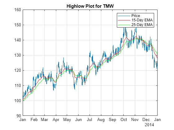
要可视化时间表数据,请使用金融图表函数,例如 highlow 或 movavg。在此示例中,移动平均线信息与 highlow 绘制在同一张图上,以提供完整的可视化信息。要获得 2014 年的股票表现,请使用 MATLAB timerange 函数选择 timetable 的行。要可视化技术指标,例如平滑异同移动平均线 (MACD),请将 timetable 对象传递给 macd 函数进行分析。
index = timerange(datetime('01-Jan-2014','Locale','en_US'),datetime('31-Dec-2014','Locale','en_US'),'closed');

highlow(TMW(index,:));
hold on

ema15 = movavg(TMW(:,'Close'),'exponential',15);
ema25 = movavg(TMW(:,'Close'),'exponential',25);

ema15 = ema15(index,:);
ema25 = ema25(index,:);
plot(ema15.Time,ema15.Close,'r');
plot(ema25.Time,ema25.Close,'g');
hold off

legend('Price','15-Day EMA','25-Day EMA')
title('Highlow Plot for TMW')
[macdLine, signalLine] = macd(TMW(:,'Close'));

plot(macdLine.Time,macdLine.Close);
hold on
plot(signalLine.Time,signalLine.Close);
hold off

title('MACD for TMW')
legend('MACD Line', 'Signal Line')

第 5 步:创建每周收益和波动率序列。
要根据每日股票价格计算每周收益,须将数据采样周期从每天变为每周。使用时间表时,请使用 MATLAB 函数 retime 或 synchronize 结合各种聚合方法计算每周的统计信息。要基于一个时间向量来调整时间表数据,请使用 retime涉及多个时间表时,需使用 synchronize。
weeklyOpen = retime(TMW(:,'Open'),'weekly','firstvalue');
weeklyHigh = retime(TMW(:,'High'),'weekly','max');
weeklyLow = retime(TMW(:,'Low'),'weekly','min');
weeklyClose = retime(TMW(:,'Close'),'weekly','lastvalue');
weeklyTMW = [weeklyOpen,weeklyHigh,weeklyLow,weeklyClose];

weeklyTMW = synchronize(weeklyTMW,TMW(:,'Volume'),'weekly','sum');
head(weeklyTMW)
       Time         Open      High      Low      Close       Volume
    ___________    ______    ______    ______    ______    __________

    02-Sep-2012       100    102.38     98.45     99.51    2.7279e+07
    09-Sep-2012     99.72    101.55     96.52     97.52    2.8518e+07
    16-Sep-2012     97.35     97.52      92.6     93.73    2.9151e+07
    23-Sep-2012     93.55     98.03     92.25     97.35     3.179e+07
    30-Sep-2012      97.3    103.15     96.68     99.66    3.3761e+07
    07-Oct-2012     99.76    106.61      98.7    104.23    3.1299e+07
    14-Oct-2012    104.54    109.75    100.55    103.77    3.1534e+07
    21-Oct-2012    103.84    104.32     96.95     97.41    3.1706e+07
要对 timetable 中的条目执行计算,请使用 MATLAB rowfun 函数,对以每周为采样周期的时间表中的每一行应用函数。
returnFunc = @(open,high,low,close,volume) log(close) - log(open);
weeklyReturn = rowfun(returnFunc,weeklyTMW,'OutputVariableNames',{'Return'});

weeklyStd = retime(TMW(:,'Close'),'weekly',@std);
weeklyStd.Properties.VariableNames{'Close'} = 'Volatility';

weeklyTMW = [weeklyReturn,weeklyStd,weeklyTMW]
weeklyTMW=208×7 timetable
       Time          Return       Volatility     Open      High      Low      Close       Volume
    ___________    ___________    __________    ______    ______    ______    ______    __________

    02-Sep-2012      -0.004912     0.59386         100    102.38     98.45     99.51    2.7279e+07
    09-Sep-2012      -0.022309     0.63563       99.72    101.55     96.52     97.52    2.8518e+07
    16-Sep-2012      -0.037894     0.93927       97.35     97.52      92.6     93.73    2.9151e+07
    23-Sep-2012       0.039817      2.0156       93.55     98.03     92.25     97.35     3.179e+07
    30-Sep-2012       0.023965      1.1014        97.3    103.15     96.68     99.66    3.3761e+07
    07-Oct-2012       0.043833      1.3114       99.76    106.61      98.7    104.23    3.1299e+07
    14-Oct-2012     -0.0073929      1.8097      104.54    109.75    100.55    103.77    3.1534e+07
    21-Oct-2012      -0.063922      2.1603      103.84    104.32     96.95     97.41    3.1706e+07
    28-Oct-2012      -0.028309      0.9815       97.45      99.1     92.58     94.73    1.9866e+07
    04-Nov-2012    -0.00010566       1.224       94.65      96.1     90.82     94.64    3.5043e+07
    11-Nov-2012       0.077244      2.4854       94.39    103.98     93.84    101.97    3.0624e+07
    18-Nov-2012       0.022823     0.55896      102.23    105.27    101.24    104.59    2.5803e+07
    25-Nov-2012      -0.012789       1.337      104.66    106.02    100.85    103.33    3.1402e+07
    02-Dec-2012      -0.043801      0.2783      103.37    103.37     97.69     98.94    3.2136e+07
    09-Dec-2012      -0.063475      1.9826       99.02     99.09     91.34     92.93    3.4447e+07
    16-Dec-2012      0.0025787      1.2789       92.95      94.2     88.58     93.19    3.3247e+07
      ⋮
另请参阅
timetable | retime | synchronize | timerange | withtol | vartype | issorted | sortrows | unique | diff | isregular | rmmissing | fillmissing