Introduction to JIPDA Smoothing
This example introduces the joint integrated probabilistic data association (JIPDA) multi-object smoothing algorithm and its applications.
Introduction
Multi-object smoothing shares a lot of common features with the multi-object tracking problem. Like a multi-object tracking algorithm, the goal of a multi-object smoothing algorithm is to estimate the number of objects and their trajectories in the presence of missed detections, false alarms, and noisy sensor observations. Most multi-object tracking algorithms are online, which means they provide an estimate at time , given measurements up to and including time step . In contrast, multi-object smoothing algorithms provide an estimate at time step , given measurements until time step , where . When is fixed to a constant representing the final time, we can further refer to such smoothing algorithms as fixed-interval smoothing algorithms. Fixed-interval multi-object smoothing algorithms can also be referred to as offline multi-object tracking algorithms, as they process recorded sensor data.
In this example, you will learn more about the JIPDA multi-object smoothing algorithm implemented by the smootherJIPDA class. JIPDA smoothing algorithm shares fundamental concepts with the JIPDA tracking algorithm. Both the JIPDA tracker and JIPDA smoother estimate probabilistic data association weights between estimated tracks and observed measurements at any given time instant. The key difference is that the smoother has access to future measurements to compute the data association, which makes it more robust to adverse events such as track breaks, track switches and so on. In the next section, you will learn how to use the smoother in MATLAB® and compare the performance of the JIPDA smoother with the JIPDA tracker.
Workflow and Comparison with Tracker
In this section, you will learn about the MATLAB workflow to use the multi-object JIPDA smoother. You will also compare the smoother results with the online tracker. To use the smoother, you begin by recording sensor data from a scenario for offline estimation. Similar to the tracker, this sensor data must be provided as a cell array of objectDetection objects. Each objectDetection object represents an object-level measurement from a sensor. For more information on how to populate sensor measurements into objectDetection format, refer to the Convert Detections to objectDetection Format example. In this section, you create these recorded detections from a simple scenario using the helper function, createSimpleScenarioData.
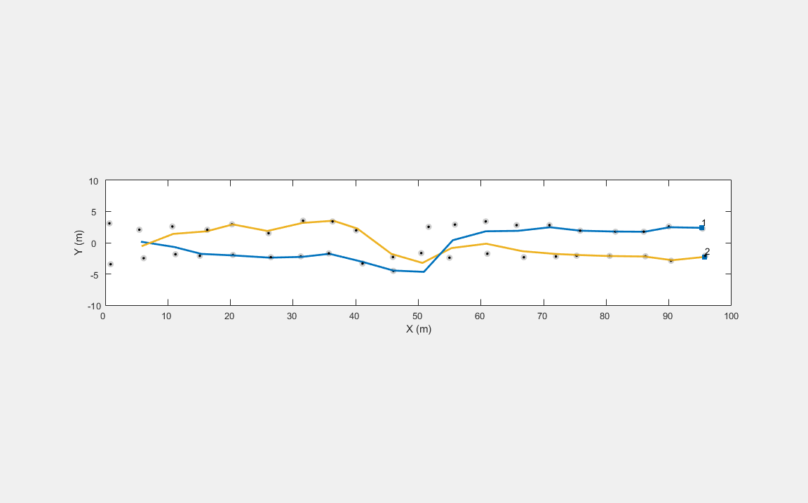
You visualize the detections using a helper class, helperJIPDASmoothingDisplay, provided with this example. In the scenario, there are two objects moving close to each other towards the positive -direction. The sensor provides Cartesian position measurements of the objects every second with an uncertainty of around 0.5 meters. Around = 40 meters, the sensor misses the top object and a false alarm is observed below the bottom object. This creates an ambiguous situation for an online tracker as it is difficult to assess whether the objects are taking a turn or if the object was missed. As this event has a low probability of occurrence, an online tracker can make a wrong decision at this step and may not be able to recover. In an offline situation, however, the smoother can assess by looking at future detection and infer that the most probable scenario is that the objects continue to move straight.
% Load detections
detectionLog = createSimpleScenarioData();

% Create figure and axes
f = figure('Units','normalized',...
    'Visible','on',...
    'Position',[0.1 0.1 0.9 0.7]);
ax = axes(f);

% Create display
display = helperJIPDASmoothingDisplay('Parent',ax,...
    'XLimits',[0 100],...
    'YLimits',[-10 10],...
    'ZLimits',[-5 5]);

% Setup display
setup(display);

% Plot detection log
display.plotDetectionHistory(detectionLog);

First, you use the online JIPDA tracker by creating a trackerJPDA object and process detections sequentially. Notice that the JIPDA tracker gets confused at the ambiguous event and is unable to recover from it, resulting in a track switching event.
% Create online JIPDA tracker
tracker = trackerJPDA(TrackLogic="Integrated");

% Run online tracker sequentially
detectionTimes = cellfun(@(x)x.Time,detectionLog);
timestamps = unique(detectionTimes)';
for time = timestamps
    tracks = tracker(detectionLog(detectionTimes == time),time);
    display.plotTrackData(tracks);
end

For offline tracking, you start by constructing a multi-object JIPDA smoother using the smootherJIPDA object. Notice that the smoother shares many properties with the JIPDA tracker. You use the smooth object function of the smoother and provide it with all the logged detections from all the time instants. The output of the smooth function represents track estimate at each time instant formatted as a cell array of objectTrack objects. The smoother is able to estimate both the number of objects and their trajectories accurately. For more details on how the smoother estimates data associations accurately, you can refer to the Understand and Analyze JIPDA Smoother Algorithm example.
smoother = smootherJIPDA
smoother =
  smootherJIPDA with properties:

                      SmootherIndex: 0
                        AnalysisFcn: ''
            FilterInitializationFcn: 'initcvekf'
                       MaxNumTracks: 100
                      MaxNumSensors: 20
                      TimeTolerance: 1.0000e-05

       DetectionAssignmentThreshold: [30 Inf]
           TrackAssignmentThreshold: 100
    MaxNumDetectionAssignmentEvents: Inf
        MaxNumTrackAssignmentEvents: Inf
            InitializationThreshold: 0

               DetectionProbability: 0.9000
                     ClutterDensity: 1.0000e-06
                   NewTargetDensity: 1.0000e-05
                          DeathRate: 0.0100
              ConfirmationThreshold: 0.9500
                  DeletionThreshold: 0.1000

                  ClassFusionMethod: 'None'
% Smooth track estimate
smoothTracks = smooth(smoother, detectionLog, timestamps);

% Display results
display.clearTrackData();
for i = 1:numel(timestamps)
    display.plotTrackData(smoothTracks{i});
end

More Examples
In this section, you will apply the multi-object JIPDA smoother to more complex scenarios with ambiguity in data associations.
Cluttered Environments
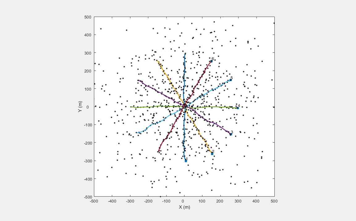
In this scenario, there are 6 objects, which move towards each other at a constant velocity and then separate from each other. Each object is detected with a probability of 0.9. In addition, there are 10 false alarms reported by the sensor every step. These random false alarms are distributed uniformly in the region. Notice that the smoother is able to estimate the trajectories of these objects accurately.
% Generate data
[detectionLog, timestamps] = createClutterData();

% Create smoother
smoother = smootherJIPDA(FilterInitializationFcn=@initcvekf, ...
    ClutterDensity=1e-6, ...
    NewTargetDensity=1e-6, ...
    DetectionAssignmentThreshold=100, ...
    TrackAssignmentThreshold=50, ...
    DetectionProbability=0.9, ...
    MaxNumDetectionAssignmentEvents=50, ...
    MaxNumTrackAssignmentEvents=100, ...
    InitializationThreshold=0, ...
    DeletionThreshold=1e-3, ...
    ConfirmationThreshold=0.95);

% Run the smoother
smoothTracks = smooth(smoother, detectionLog, timestamps);

% Visualize results
display.Parent.XLim = [-500 500];
display.Parent.YLim = [-500 500];
display.Parent.ZLim = [-150 -50];

display.plotDetectionHistory(detectionLog);
display.clearTrackData();
for i = 1:numel(timestamps)
    display.plotTrackData(smoothTracks{i});
end

Classification-Aided Smoothing
In this section, you perform smoothing with classified detections using the data from Classification-Aided Tracking section of the Introduction to Class Fusion and Classification-Aided Tracking Example. The detections and tracks are visualized in different colors for each class. Notice that the trajectories and the class of the tracks are estimated correctly by the smoother.
% Load data
load("classAidedScenarioData.mat","allData");
detectionLog = [allData.Detections];
timestamps = [allData.Time];

% Create smoother
smoother = smootherJIPDA(DetectionAssignmentThreshold = 1000,...
    TrackAssignmentThreshold = 1000,...
    ClutterDensity=1e-8,...
    MaxNumDetectionAssignmentEvents=50,...
    MaxNumTrackAssignmentEvents=250,...
    NewTargetDensity=1e-8,...
    FilterInitializationFcn=@initcvekf,...
    ClassFusionMethod="Bayes",...
    DetectionAssignmentClassWeight=0.5,...
    TrackAssignmentClassWeight=0.5,...
    DeletionThreshold=1e-2,...
    ConfirmationThreshold=0.5,...
    InitialClassProbabilities= [0.25 0.25 0.25 0.25]);

% Estimate tracks
smoothTracks = smooth(smoother, detectionLog, timestamps);

% Set new limits
display.Parent.XLim = [-3500 1500];
display.Parent.YLim = [0 8000];
display.Parent.ZLim = [-1e3 1e3];

% Clear old data
display.clearDetectionData();
display.clearTrackData();

% Visualize results
display.plotClassifiedDetectionHistory(detectionLog);
for i = 1:numel(timestamps)
    display.plotClassifiedTrack(smoothTracks{i});
end

Summary
In this example, you use multi-object smoothing for offline estimation of number of objects and their trajectories. Some applications of multi-object smoothing include ground truth estimation from recorded real-world sensor data. You can further use the ground truth estimate to assess the performance of an online tracking algorithm. You can also use the ground truth estimate to recreate a scenario and generate simulated variants of the sensor data. For an application of multi-object smoothing with lidar and camera, refer to the Fuse Prerecorded Lidar and Camera Data to Generate Vehicle Track List for Scenario Generation (Automated Driving Toolbox) example.
References
[1] Song, Taek Lyul, and Darko Mušicki. "Smoothing innovations and data association with IPDA." Automatica 48.7 (2012): 1324-1329.
[2] Kim, Tae Han, et al. "Smoothing joint integrated probabilistic data association." IET Radar, Sonar & Navigation 9.1 (2015): 62-66.
[3] Memon, Sufyan, Won Jun Lee, and Taek Lyul Song. "Efficient smoothing for multiple maneuvering targets in heavy clutter." 2016 International Conference on Control, Automation and Information Sciences (ICCAIS). IEEE, 2016.
Supporting Functions
createSimpleScenarioData
function [detectionLog, timestamps] = createSimpleScenarioData()
% Random seed for reproducible data
rng(1);

% timestamps
timestamps = 1:20;

% True X Position
x = 1:5:100;

% True Y Position
y = 2.5*ones(1,20);

% True Z Position
z = zeros(1,20);

% Append for both objects
x = [x x];
y = [y -y];
z = [z z];
timestamps = [timestamps timestamps];

% Add noise
meas = [x;y;z] + 0.5*randn(3,40);

% Missed object at t = 10
meas(:,10) = [];
timestamps(10) = [];

% False alarm at t = 10
meas(:,end+1) = [x(10);-4.5;0];
timestamps(end+1) = 10;

% Assemble using objectDetection
detectionLog = cell(size(meas,2),1);
for i = 1:size(meas,2)
    detectionLog{i} = objectDetection(timestamps(i),meas(:,i),"MeasurementNoise",0.25*eye(3));
end
end
createClutterData
function [detectionLog, timestamps] = createClutterData()
% Reproducible seed
rng(1);

% Create Scenario
scenario = trackingScenario;
scenario.StopTime = 120;
scenario.UpdateRate = 0.5;

% Add platforms
theta = linspace(90,270,7);
for i = 1:6
    p = platform(scenario);
    p.Trajectory.Position = [300*cosd(theta(i)) 300*sind(theta(i)) -100];
    p.Trajectory.Velocity = -[5*cosd(theta(i)) 5*sind(theta(i)) 0];
end

% Log detections for offline estimation
detectionLog = cell(0,1);
timestamps = zeros(0,1);

% Estimate and visualize online tracks
while advance(scenario)
    % Current time
    time = scenario.SimulationTime;

    % Ground truth
    gTruth = platformPoses(scenario);

    % Detections with clutter
    detections = createDetections(gTruth, time);

    % Log
    detectionLog = [detectionLog;detections]; %#ok<AGROW>
    timestamps = [timestamps;time]; %#ok<AGROW>
end
end

function detections = createDetections(gTruth,time)
% True detections from objects with Pd = 0.9
detections = cell(0,1);
for i = 1:numel(gTruth)
    if rand < 0.9
        detections{end+1,1} = objectDetection(time,gTruth(i).Position(:) + 5*randn(3,1),"MeasurementNoise",25*eye(3),"ObjectAttributes",struct);
    end
end
% 10 false alarms per step
nFalse = 10;
for i = 1:nFalse
    detections{end+1,1} = objectDetection(time,[250*randn 250*randn -100]' + 5*randn(3,1),"MeasurementNoise",25*eye(3),"ObjectAttributes",struct);
end
end