使用基于问题的遗传算法解决混合整数工程设计问题

此示例说明如何使用 Global Optimization Toolbox 中的遗传算法(ga)求解器解决混合整数工程设计问题。该示例采用基于问题的方法。对于使用基于求解器的方法的版本，请参阅使用遗传算法解决混合整数工程设计问题。

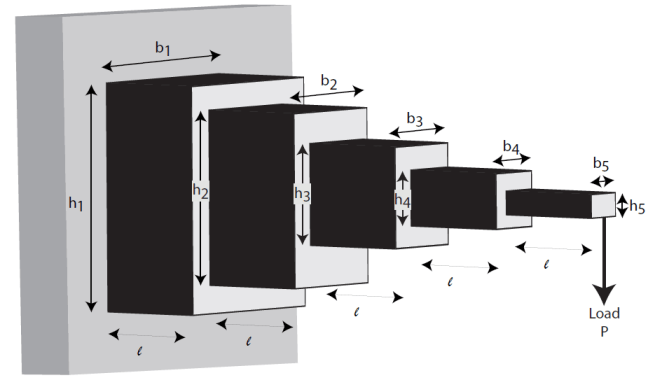
本例所说明的问题涉及阶梯悬臂梁的设计。具体来说，梁必须能够承载规定的端部载荷。优化问题是在各种工程设计约束下最小化梁体积。

Thanedar 和 Vanderplaats [1] 描述了这个问题。

阶梯式悬臂梁设计问题

阶梯悬臂梁的一端受到支撑，在自由端施加载荷，如下图所示。梁必须能够在距支撑件固定距离 $P$ 处支撑给定的负载 $L$ 。梁的设计者可以改变每个台阶或部分的宽度（ $b_{i}$ ）和高度（ $h_{i}$ ）。悬臂的每个部分具有相同的长度， $l = L_{1}$ 。

梁的体积

梁 $V$ 的体积是个体部分体积的总和。

$V = l (b_{1} h_{1} + b_{2} h_{2} + b_{3} h_{3} + b_{4} h_{4} + b_{5} h_{5})$ .

设计约束：弯曲应力

考虑单悬臂梁，其坐标中心位于梁自由端横截面的中心。梁中点 $(x, y, z)$ 处的弯曲应力由下式给出

$σ_{b} = M (x) y / I$ ,

其中 $M (x)$ 是 $x$ 处的弯矩， $x$ 是距端部载荷的距离， $I$ 是梁的面积惯性矩。

图中所示的阶梯悬臂梁中，梁各截面的最大弯矩为 $P D_{i}$ ，其中 $D_{i}$ 为梁各截面距端部荷载的最大距离 $P$ 。因此，梁 $σ_{i}$ 第 i 段的最大应力由下式给出：

$σ_{i} = P D_{i} (h_{i} / 2) / I_{i}$ ,

最大应力发生在梁的边缘， $y = h_{i} / 2$ 。梁的第 i 个截面的面积惯性矩由下式给出：

$I_{i} = b_{i} h_{i}^{3} / 12$ .

将此表达式代入 $σ_{i}$ 方程可得出

$σ_{i} = 6 P D_{i} / b_{i} h_{i}^{2}$ .

悬臂各部分的弯曲应力不得超过最大允许应力 $σ_{m a x}$ 。因此，五个弯曲应力约束（悬臂的每个台阶一个）为：

$\frac{6 P l}{b_{5} h_{5}^{2}} \leq σ_{m a x}$

$\frac{6 P (2 l)}{b_{4} h_{4}^{2}} \leq σ_{m a x}$

$\frac{6 P (3 l)}{b_{3} h_{3}^{2}} \leq σ_{m a x}$

$\frac{6 P (4 l)}{b_{2} h_{2}^{2}} \leq σ_{m a x}$

$\frac{6 P (5 l)}{b_{1} h_{1}^{2}} \leq σ_{m a x}$

设计约束：端部挠度

您可以使用卡斯蒂利亚诺第二定理计算悬臂的末端挠度，该定理指出

$δ = \frac{\partial U}{\partial P}$ ,

其中 $δ$ 是梁的挠度， $U$ 是由于施加的力 $P$ 而储存在梁中的能量。

悬臂梁中存储的能量由下式给出：

$U = \int_{0}^{L} M^{2} / 2 E I d x$ ,

其中 $M$ 是在 $x$ 处施加力的矩。

鉴于悬臂梁的 $M = P x$ ，您可以将上述方程写为

$U = P^{2} / 2 E \int_{0}^{l} [(x + 4 l)^{2} / I_{1} + (x + 3 l)^{2} / I_{2} + (x + 2 l)^{2} / I_{3} + (x + l)^{2} / I_{4} + x^{2} / I_{5}] d x$ ,

其中 $I_{n}$ 是悬臂第 n 部分的面积惯性矩。计算积分可得出 $U$ 的表达式

$U = (P^{2} / 2) (l^{3} / 3 E) (61 / I_{1} + 37 / I_{2} + 19 / I_{3} + 7 / I_{4} + 1 / I_{5})$ .

应用卡斯蒂利亚诺定理，梁的端部挠度由下式给出

$δ = P l^{3} / 3 E (61 / I_{1} + 37 / I_{2} + 19 / I_{3} + 7 / I_{4} + 1 / I_{5})$ .

悬臂的端部挠度 $δ$ 必须小于最大允许挠度 $δ_{m a x}$ ，从而给出约束

$P l^{3} / 3 E (61 / I_{1} + 37 / I_{2} + 19 / I_{3} + 7 / I_{4} + 1 / I_{5}) \leq δ_{m a x}$ .

设计约束：纵横比

对于悬臂的每一步，纵横比不得超过最大允许纵横比 $a_{m a x}$ 。即：

$h_{i} / b_{i} \leq a_{m a x}$ ，其中 $i = 1, . . ., 5$ 。

设计约束：边界和整数约束

梁的第一步只能加工到最接近厘米的精度。也就是说， $b_{1}$ 和 $h_{1}$ 必须是整数。其余变量是连续的。变量的边界是：

$1 \leq b_{1} \leq 5$

$30 \leq h_{1} \leq 65$

$2.4 \leq b_{2}, b_{3} \leq 3.1$

$45 \leq h_{2}, h_{3} \leq 60$

$1 \leq b_{4}, b_{5} \leq 5$

$30 \leq h_{4}, h_{5} \leq 65$

此问题的设计参数

对于本例中的问题，梁必须支撑的端部载荷是 $P = 50000 N$ 。

梁长度和最大端部挠度为：

梁总长度， $L = 500 c m$
梁的个体部分的长度， $l = L_{1} = 100 c m$
最大梁端挠度， $δ_{m a x} = 2.7 c m$

梁每一步允许的最大应力为 $σ_{m a x} = 14000 N / c m^{2}$ 。

梁每一步的杨氏模量为 $E = 2 \times 1 0^{7} N / c m^{2}$ 。

基于问题的设置

为该问题创建优化变量。梁第一部分的宽度和高度变量是整数类型，因此必须与其他四个连续的变量分开创建它们。

b1 = optimvar("b1","Type","integer","LowerBound",1,"UpperBound",5);
h1 = optimvar("h1","Type","integer","LowerBound",30,"UpperBound",65);
bc = optimvar("bc",4,"LowerBound",[2.4 2.4 1 1],"UpperBound",[3.1 3.1 5 5]);
hc = optimvar("hc",4,"LowerBound",[45 45 30 30],"UpperBound",[60 60 65 65]);

为了方便起见，将高度和宽度变量放入单个变量中。然后您可以根据这些变量轻松地表达目标和约束。

h = [h1;hc];
b = [b1;bc];

创建一个优化问题，以梁的体积为目标函数，其中梁的每个步骤（或部分）长为 $L_{1} = 100$ 厘米：体积 = $L_{1} \sum h_{i} w_{i}$ 。

L_1 = 100; % Length of each step of the cantilever
prob = optimproblem("Objective",L_1*dot(h,b));

对压力施加约束。

P = 50000; % End load
E = 2e7; % Young's modulus in N/cm^2
deltaMax = 2.7; % Maximum end deflection
sigmaMax = 14000; % Maximum stress in each section of the beam
aMax = 20; % Maximum aspect ratio in each section of the beam

stress = 6*P*L_1./(b.*(h.^2));
stepnum = (5:-1:1)';
stress = stress.*stepnum;
prob.Constraints.stress = stress <= sigmaMax;

创建对挠度的约束。

deflectionMultiplier = (P*L_1^3/E)*[244 148 76 28 4];
bh3 = 1./(b.*(h.^3));
prob.Constraints.deflection = deflectionMultiplier*bh3 <= deltaMax;

创建纵横比的约束。

prob.Constraints.aspect = h <= aMax*b;

检查问题设置。

show(prob)

  OptimizationProblem : 

	Solve for:
       b1, bc, h1, hc
	where:
       b1, h1 integer
	minimize :
       100*h1*b1 + 100*hc(1)*bc(1) + 100*hc(2)*bc(2) + 100*hc(3)*bc(3) + 100*hc(4)*bc(4)


	subject to stress:
       arg_LHS <= arg_RHS

       where:

             arg2 = zeros(5, 1);
             arg1 = zeros(5, 1);
             arg1(1) = h1;
             arg1(2:5) = hc;
             arg2(1) = b1;
             arg2(2:5) = bc;
             arg_LHS = ((30000000 ./ (arg2(:) .* arg1(:).^2)) .* extraParams{1});
             arg2 = 14000;
             arg1 = arg2(ones(1,5));
             arg_RHS = arg1(:);

       extraParams

	subject to deflection:
       arg_LHS <= 2.7

       where:

             arg2 = zeros(5, 1);
             arg1 = zeros(5, 1);
             arg1(1) = h1;
             arg1(2:5) = hc;
             arg2(1) = b1;
             arg2(2:5) = bc;
             arg_LHS = (extraParams{1} * (1 ./ (arg2(:) .* arg1(:).^3)));

       extraParams

	subject to aspect:
       -20*b1 + h1 <= 0
       -20*bc(1) + hc(1) <= 0
       -20*bc(2) + hc(2) <= 0
       -20*bc(3) + hc(3) <= 0
       -20*bc(4) + hc(4) <= 0

	variable bounds:
       1 <= b1 <= 5

       2.4 <= bc(1) <= 3.1
       2.4 <= bc(2) <= 3.1
         1 <= bc(3) <=   5
         1 <= bc(4) <=   5

       30 <= h1 <= 65

       45 <= hc(1) <= 60
       45 <= hc(2) <= 60
       30 <= hc(3) <= 65
       30 <= hc(4) <= 65

求解问题

设置选项以使用中等规模 150、中等最大代数 400、略大于默认精英计数 10、较小函数容差 1e-8，以及显示迭代过程中函数值的绘图函数。

opts = optimoptions(@ga, ...
                    'PopulationSize', 150, ...
                    'MaxGenerations', 400, ...
                    'EliteCount', 10, ...
                    'FunctionTolerance', 1e-8, ...
                    'PlotFcn', @gaplotbestf);

解决问题，指定 ga 求解器和选项。

rng default % For reproducibility
[sol,fval,exitflag] = solve(prob,"Solver","ga","Options",opts)

Solving problem using ga.

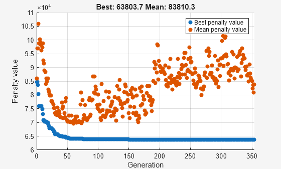
Figure Genetic Algorithm contains an axes object. The axes object with title Best: 63803.7 Mean: 83810.3, xlabel Generation, ylabel Penalty value contains 2 objects of type scatter. These objects represent Best penalty value, Mean penalty value.

ga stopped because the average change in the penalty function value is less than options.FunctionTolerance and 
the constraint violation is less than options.ConstraintTolerance.

sol = struct with fields:
    b1: 3
    bc: [4×1 double]
    h1: 60
    hc: [4×1 double]

fval = 
6.3804e+04

exitflag = 
    SolverConvergedSuccessfully

查看解变量及其边界。

widths = [sol.b1;sol.bc];
heights = [sol.h1;sol.hc];
widthbounds = [b1.LowerBound b1.UpperBound;
    bc.LowerBound bc.UpperBound];
heightbounds = [h1.LowerBound h1.UpperBound;
    hc.LowerBound hc.UpperBound];
T = table(widths,heights,widthbounds,heightbounds,...
    'VariableNames',["Width" "Height" "Width Bounds" "Height Bounds"])

T=5×4 table
    Width     Height    Width Bounds    Height Bounds
    ______    ______    ____________    _____________

         3        60       1      5       30    65   
    2.9063    54.983     2.4    3.1       45    60   
    2.5805    51.609     2.4    3.1       45    60   
    2.2785    45.565       1      5       30    65   
    1.7502    34.991       1      5       30    65

该解不在任何边界上。按照规定，第一个解变量是整数值。

添加离散非整数约束约束

假设工程师了解到悬臂的第二步和第三步的宽度和高度只能从标准集合中选择。增加这个约束后，该问题与 [1] 中解决的问题相同。

首先，描述要添加到优化中的额外约束：

梁的第二和第三台阶的宽度必须从 [2.4, 2.6, 2.8, 3.1] cm 中选择。
梁的第二和第三踏步高度必须从 [45, 50, 55, 60] 厘米中选择。

为了解决这个问题，需要将变量 $w c (1)$ 、 $w c (2)$ 、 $h c (1)$ 和 $h c (2)$ 指定为离散变量。理想情况下，您应该使用 $S (x_{j})$ 作为离散值，其中 $S$ 表示允许的值集，而 $x_{j}$ 表示问题变量。但是，您不能使用优化变量作为索引。您可以通过调用 fcn2optimexpr 来解决此问题。

widthlist = [2.4,2.6,2.8,3.1];
heightlist = [45 50 55 60];
b23 = optimvar("w23",2,"Type","integer",...
    "LowerBound",1,"UpperBound",length(widthlist));
h23 = optimvar("h23",2,"Type","integer",...
    "LowerBound",1,"UpperBound",length(heightlist));
b45 = optimvar("b45",2,"LowerBound",1,"UpperBound",5);
h45 = optimvar("h45",2,"LowerBound",30,"UpperBound",65);
% Preferred syntax is we = [widthlist(b23(1));widthlist(b23(2))];
% However, this syntax is illegal.
% Instead call fcn2optimexpr.
we = fcn2optimexpr(@(x)[widthlist(x(1));widthlist(x(2))],b23);
he = fcn2optimexpr(@(x)[heightlist(x(1));heightlist(x(2))],h23);

与之前一样，创建表达式 b 和 h 来表示变量。

b = [b1;we;b45];
h = [h1;he;h45];

问题表述的其余部分与之前相同。

prob2 = optimproblem("Objective",L_1*dot(h,b));

对压力施加约束。

stress = 6*P*L_1./(b.*(h.^2));
stepnum = (5:-1:1)';
stress = stress.*stepnum;
prob2.Constraints.stress = stress <= sigmaMax;

创建对挠度的约束。

deflectionMultiplier = (P*L_1^3/E)*[244 148 76 28 4];
bh3 = 1./(b.*(h.^3));
prob2.Constraints.deflection = deflectionMultiplier*bh3 <= deltaMax;

创建纵横比的约束。

prob2.Constraints.aspect = h <= aMax*b;

检查问题设置。

show(prob2)

  OptimizationProblem : 

	Solve for:
       b1, b45, h1, h23, h45, w23
	where:
       b1, h1, h23, w23 integer
	minimize :
       (100 .* (arg2(:).' * arg4(:)))

       where:

           arg4 = zeros(5, 1);
           arg2 = zeros(5, 1);
           anonymousFunction2 = @(x)[heightlist(x(1));heightlist(x(2))];
           arg1 = anonymousFunction2(h23);
           arg2(1) = h1;
           arg2(2:3) = arg1;
           arg2(4:5) = h45;
           anonymousFunction1 = @(x)[widthlist(x(1));widthlist(x(2))];
           arg3 = anonymousFunction1(w23);
           arg4(1) = b1;
           arg4(2:3) = arg3;
           arg4(4:5) = b45;


	subject to stress:
       arg_LHS <= arg_RHS

       where:

             arg4 = zeros(5, 1);
             arg2 = zeros(5, 1);
             anonymousFunction2 = @(x)[heightlist(x(1));heightlist(x(2))];
             arg1 = anonymousFunction2(h23);
             arg2(1) = h1;
             arg2(2:3) = arg1;
             arg2(4:5) = h45;
             anonymousFunction1 = @(x)[widthlist(x(1));widthlist(x(2))];
             arg3 = anonymousFunction1(w23);
             arg4(1) = b1;
             arg4(2:3) = arg3;
             arg4(4:5) = b45;
             arg_LHS = ((30000000 ./ (arg4(:) .* arg2(:).^2)) .* extraParams{1});
             arg2 = 14000;
             arg1 = arg2(ones(1,5));
             arg_RHS = arg1(:);

       extraParams

	subject to deflection:
       arg_LHS <= 2.7

       where:

             arg4 = zeros(5, 1);
             arg2 = zeros(5, 1);
             anonymousFunction2 = @(x)[heightlist(x(1));heightlist(x(2))];
             arg1 = anonymousFunction2(h23);
             arg2(1) = h1;
             arg2(2:3) = arg1;
             arg2(4:5) = h45;
             anonymousFunction1 = @(x)[widthlist(x(1));widthlist(x(2))];
             arg3 = anonymousFunction1(w23);
             arg4(1) = b1;
             arg4(2:3) = arg3;
             arg4(4:5) = b45;
             arg_LHS = (extraParams{1} * (1 ./ (arg4(:) .* arg2(:).^3)));

       extraParams

	subject to aspect:
       arg_LHS <= arg_RHS

       where:

             arg1 = zeros(5, 1);
             arg1(1) = h1;
             anonymousFunction2 = @(x)[heightlist(x(1));heightlist(x(2))];
             arg2 = anonymousFunction2(h23);
             arg1(2:3) = arg2;
             arg1(4:5) = h45;
             arg_LHS = arg1(:);
             arg2 = zeros(5, 1);
             anonymousFunction1 = @(x)[widthlist(x(1));widthlist(x(2))];
             arg1 = anonymousFunction1(w23);
             arg2(1) = b1;
             arg2(2:3) = arg1;
             arg2(4:5) = b45;
             arg_RHS = (20 .* arg2(:));

	variable bounds:
       1 <= b1 <= 5

       1 <= b45(1) <= 5
       1 <= b45(2) <= 5

       30 <= h1 <= 65

       1 <= h23(1) <= 4
       1 <= h23(2) <= 4

       30 <= h45(1) <= 65
       30 <= h45(2) <= 65

       1 <= w23(1) <= 4
       1 <= w23(2) <= 4

解决离散约束约束问题

解决问题，指定 ga 求解器和选项。

rng default % For reproducibility
[sol2,fval2,exitflag2] = solve(prob2,"Solver","ga","Options",opts)

Solving problem using ga.

Figure Genetic Algorithm contains an axes object. The axes object with title Best: 64803.2 Mean: 69025.3, xlabel Generation, ylabel Penalty value contains 2 objects of type scatter. These objects represent Best penalty value, Mean penalty value.

ga stopped because it exceeded options.MaxGenerations.

sol2 = struct with fields:
     b1: 3
    b45: [2×1 double]
     h1: 60
    h23: [2×1 double]
    h45: [2×1 double]
    w23: [2×1 double]

fval2 = 
6.4803e+04

exitflag2 = 
    SolverLimitExceeded

目标值会增加，因为增加约束只能增加目标。

查看解并将其与其边界进行比较。

widths = [sol2.b1;widthlist(sol2.w23(1));widthlist(sol2.w23(2));sol2.b45];
heights = [sol2.h1;heightlist(sol2.h23(1));heightlist(sol2.h23(2));sol2.h45];
widthbounds = [b1.LowerBound b1.UpperBound;
    widthlist(1) widthlist(end);
     widthlist(1) widthlist(end);
    b45.LowerBound b45.UpperBound];
heightbounds = [h1.LowerBound h1.UpperBound;
     heightlist(1) heightlist(end);
     heightlist(1) heightlist(end);
    h45.LowerBound h45.UpperBound];
T = table(widths,heights,widthbounds,heightbounds,...
    'VariableNames',["Width" "Height" "Width Bounds" "Height Bounds"])

T=5×4 table
    Width     Height    Width Bounds    Height Bounds
    ______    ______    ____________    _____________

         3        60       1      5       30    65   
       3.1        55     2.4    3.1       45    60   
       2.6        50     2.4    3.1       45    60   
     2.286     45.72       1      5       30    65   
    1.8532    34.004       1      5       30    65

唯一处于边界内的解变量是第二部分的宽度，其最大值为 3.1。

参考资料

[1] Thanedar, P. B., and G. N. Vanderplaats."Survey of Discrete Variable Optimization for Structural Design." Journal of Structural Engineering 121 (3), 1995, pp. 301–306.

另请参阅

ga | fcn2optimexpr | solve

主题

使用遗传算法解决混合整数工程设计问题