Quantize Layers in Object Detectors and Generate CUDA Code

This example uses:

This example shows how to generate CUDA® code for an SSD vehicle detector and a YOLO v2 vehicle detector that performs inference computations in 8-bit integers for the convolutional layers.

Deep learning is a powerful machine learning technique in which you train a network to learn image features and perform detection tasks. There are several techniques for object detection using deep learning, such as Faster R-CNN, You Only Look Once (YOLO v2), and SSD. For more information, see Object Detection Using YOLO v2 Deep Learning (Computer Vision Toolbox) and Object Detection Using SSD Deep Learning (Computer Vision Toolbox).

Neural network architectures used for deep learning applications contain many processing layers, including convolutional layers. Deep learning models typically work on large sets of labeled data. Performing inference on these models is computationally intensive, consuming significant amounts of memory. Neural networks use memory to store input data, parameters (weights), and activations from each layer as the input propagates through the network. Deep neural networks trained in MATLAB® use single-precision floating point data types. Even networks that are small in size require a considerable amount of memory and hardware to perform these floating-point arithmetic operations. These restrictions can inhibit deployment of deep learning models to devices that have low computational power and smaller memory resources. By using a lower precision to store the weights and activations, you can reduce the memory requirements of the network.

You can use Deep Learning Toolbox™ in tandem with the Deep Learning Toolbox Model Quantization Library support package to reduce the memory footprint of a deep neural network by quantizing the weights, biases, and activations of convolution layers to 8-bit scaled integer data types. Then, you can use GPU Coder™ to generate CUDA code for the optimized network.

Download Pretrained Network

Download a pretrained object detector to avoid having to wait for training to complete.

detectorType = 2

detectorType = 2

switch detectorType
    case 1
        if ~exist('ssdResNet50VehicleExample_20a.mat','file')
            disp('Downloading pretrained detector...');
            pretrainedURL = 'https://www.mathworks.com/supportfiles/vision/data/ssdResNet50VehicleExample_20a.mat';
            websave('ssdResNet50VehicleExample_20a.mat',pretrainedURL);
        end
    case 2
        if ~exist('yolov2ResNet50VehicleExample_19b.mat','file')    
            disp('Downloading pretrained detector...');
            pretrainedURL = 'https://www.mathworks.com/supportfiles/vision/data/yolov2ResNet50VehicleExample_19b.mat';
            websave('yolov2ResNet50VehicleExample_19b.mat',pretrainedURL);
        end
end

Load Data

This example uses a small vehicle data set that contains 295 images. Many of these images come from the Caltech Cars 1999 and 2001 data sets, created by Pietro Perona and used with permission. Each image contains one or two labeled instances of a vehicle. A small data set is useful for exploring the training procedure, but in practice, more labeled images are needed to train a robust detector. Extract the vehicle images and load the vehicle ground truth data.

unzip vehicleDatasetImages.zip
data = load('vehicleDatasetGroundTruth.mat');
vehicleDataset = data.vehicleDataset;

Prepare Data for Training, Calibration, and Validation

The training data is stored in a table. The first column contains the path to the image files. The remaining columns contain the ROI labels for vehicles. Display the first few rows of the data.

vehicleDataset(1:4,:)

ans=4×2 table
              imageFilename                   vehicle     
    _________________________________    _________________

    {'vehicleImages/image_00001.jpg'}    {[220 136 35 28]}
    {'vehicleImages/image_00002.jpg'}    {[175 126 61 45]}
    {'vehicleImages/image_00003.jpg'}    {[108 120 45 33]}
    {'vehicleImages/image_00004.jpg'}    {[124 112 38 36]}

Split the data set into training, validation, and test sets. Select 60% of the data for training, 10% for calibration, and the remainder for validating the trained detector.

rng(0);
shuffledIndices = randperm(height(vehicleDataset));
idx = floor(0.6 * length(shuffledIndices) );

trainingIdx = 1:idx;
trainingDataTbl = vehicleDataset(shuffledIndices(trainingIdx),:);

calibrationIdx = idx+1 : idx + 1 + floor(0.1 * length(shuffledIndices) );
calibrationDataTbl = vehicleDataset(shuffledIndices(calibrationIdx),:);

validationIdx = calibrationIdx(end)+1 : length(shuffledIndices);
validationDataTbl = vehicleDataset(shuffledIndices(validationIdx),:);

Use imageDatastore and boxLabelDatastore to create datastores for loading the image and label data during training and evaluation.

imdsTrain = imageDatastore(trainingDataTbl{:,'imageFilename'});
bldsTrain = boxLabelDatastore(trainingDataTbl(:,'vehicle'));

imdsCalibration = imageDatastore(calibrationDataTbl{:,'imageFilename'});
bldsCalibration = boxLabelDatastore(calibrationDataTbl(:,'vehicle'));

imdsValidation = imageDatastore(validationDataTbl{:,'imageFilename'});
bldsValidation = boxLabelDatastore(validationDataTbl(:,'vehicle'));

Combine the image and box label datastores.

trainingData = combine(imdsTrain,bldsTrain);
calibrationData = combine(imdsCalibration,bldsCalibration);
validationData = combine(imdsValidation,bldsValidation);

Display one of the training images and box labels.

data = read(calibrationData);
I = data{1};
bbox = data{2};
annotatedImage = insertShape(I,'Rectangle',bbox);
annotatedImage = imresize(annotatedImage,2);
figure
imshow(annotatedImage)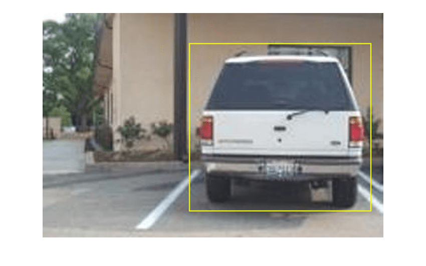

Define Network Parameters

To reduce the computational cost of running the example, specify a network input size that corresponds to the minimum size required to run the network.

inputSize = []; 
switch detectorType 
    case 1
        inputSize = [300 300 3]; % Minimum size for SSD
    case 2
        inputSize = [224 224 3]; % Minimum size for YOLO v2
end

Define the number of object classes to detect.

numClasses = width(vehicleDataset)-1;

Data Augmentation

Data augmentation is used to improve network accuracy by randomly transforming the original data during training. By using data augmentation, you can add more variety to the training data without actually having to increase the number of labeled training samples.

Use transformations to augment the training data by:

Randomly flipping the image and associated box labels horizontally.
Randomly scaling the image and associated box labels.
Jitter the image color.

Note that data augmentation is not applied to the test data. Ideally, test data is representative of the original data and left unmodified for unbiased evaluation.

augmentedCalibrationData = transform(calibrationData,@augmentVehicleData);

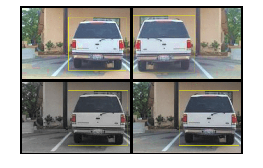
Visualize augmented training data by reading the same image multiple times.

augmentedData = cell(4,1);
for k = 1:4
    data = read(augmentedCalibrationData);
    augmentedData{k} = insertShape(data{1},'Rectangle',data{2});
    reset(augmentedCalibrationData);
end

figure
montage(augmentedData,'BorderSize',10)

Preprocess Calibration Data

Preprocess the augmented calibration data to prepare for calibration of the network.

preprocessedCalibrationData = transform(augmentedCalibrationData,@(data)preprocessVehicleData(data,inputSize));

Read the preprocessed calibration data.

data = read(preprocessedCalibrationData);

Display the image and bounding boxes.

I = data{1};
bbox = data{2};
annotatedImage = insertShape(I,'Rectangle',bbox);
annotatedImage = imresize(annotatedImage,2);
figure
imshow(annotatedImage)

Load and Test Pretrained Detector

Load the pretrained detector.

switch detectorType
    case 1
        % Load pretrained SSD detector for the example.
        pretrained = load('ssdResNet50VehicleExample_20a.mat');
        detector = pretrained.detector;
    case 2 
        % Load pretrained YOLO v2 detector for the example.
        pretrained = load('yolov2ResNet50VehicleExample_19b.mat');
        detector = pretrained.detector;
end

As a quick test, run the detector on one test image.

data = read(calibrationData);
I = data{1,1};
I = imresize(I,inputSize(1:2));
[bboxes,scores] = detect(detector,I, 'Threshold', 0.4);

Display the results.

I = insertObjectAnnotation(I,'rectangle',bboxes,scores);
figure
imshow(I)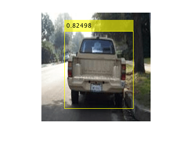

Validate Floating-Point Network

Evaluate the trained object detector on a large set of images to measure the performance. Use the evaluateObjectDetection (Computer Vision Toolbox) function to measure common object detector metrics, such as average precision and log-average miss rates. For this example, use the average precision metric to evaluate performance. The average precision provides a single number that incorporates the ability of the detector to make correct classifications (precision) and the ability of the detector to find all relevant objects (recall).

Apply the same preprocessing transform to the test data as for the training data. Note that data augmentation is not applied to the test data. Ideally, test data is representative of the original data and left unmodified for unbiased evaluation.

preprocessedValidationData = transform(validationData,@(data)preprocessVehicleData(data,inputSize));

Run the detector on all the test images.

detectionResults = detect(detector, preprocessedValidationData,'Threshold',0.4);

Evaluate the object detector using average precision metric.

metrics = evaluateObjectDetection(detectionResults,preprocessedValidationData);
ap = averagePrecision(metrics,ClassName="vehicle");
[precision, recall] = precisionRecall(metrics,ClassName="vehicle");
precision = precision{:};
recall = recall{:};

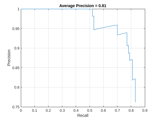
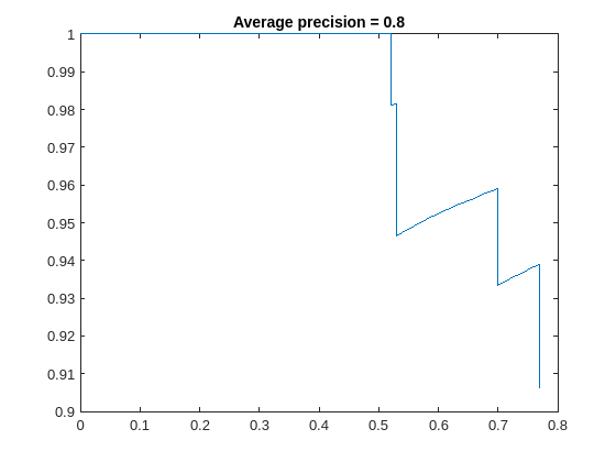
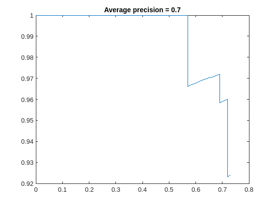
The precision/recall (PR) curve highlights how precise a detector is at varying levels of recall. Ideally, the precision is 1 at all recall levels. Using more data can help improve the average precision, but might require more training time. Plot the PR curve.

figure
plot(recall,precision)
xlabel('Recall')
ylabel('Precision')
grid on
title(sprintf('Average Precision = %.2f',ap))

Generate Calibration Result File for the Network

Create a dlquantizer object and specify the detector to quantize. By default, the execution environment is set to GPU. To learn about the products required to quantize and deploy the detector to a GPU environment, see Quantization Workflow Prerequisites (Deep Learning Toolbox). Note that code generation does not support quantized deep neural networks produced by the quantize (Deep Learning Toolbox) function.

quantObj = dlquantizer(detector)

quantObj = 
  dlquantizer with properties:

           NetworkObject: [1×1 yolov2ObjectDetector]
    ExecutionEnvironment: 'GPU'

Specify the metric function in a dlquantizationOptions object.

quantOpts = dlquantizationOptions;
quantOpts = dlquantizationOptions('Target','gpu', ...
    'MetricFcn', ...
    {@(x)hVerifyDetectionResults(x, detector.Network, preprocessedValidationData)});

Use the calibrate function to exercise the network with sample inputs and collect range information. The calibrate function exercises the network and collects the dynamic ranges of the weights and biases in the convolution and fully connected layers of the network, as well as the dynamic ranges of the activations in all layers of the network. The function returns a table. Each row of the table contains range information for a learnable parameter of the optimized network.

calResults = calibrate(quantObj,preprocessedCalibrationData)

calResults=202×5 table
       Optimized Layer Name       Network Layer Name    Learnables / Activations    MinValue    MaxValue
    __________________________    __________________    ________________________    ________    ________

    {'conv1_Weights'         }    {'conv1'         }           "Weights"             -9.3984      9.511 
    {'conv1_Bias'            }    {'conv1'         }           "Bias"                -2.6468     6.3474 
    {'res2a_branch2a_Weights'}    {'res2a_branch2a'}           "Weights"            -0.85967    0.35191 
    {'res2a_branch2a_Bias'   }    {'res2a_branch2a'}           "Bias"                -5.0999     5.6429 
    {'res2a_branch2b_Weights'}    {'res2a_branch2b'}           "Weights"            -0.24903    0.32103 
    {'res2a_branch2b_Bias'   }    {'res2a_branch2b'}           "Bias"                 -2.749     5.1706 
    {'res2a_branch2c_Weights'}    {'res2a_branch2c'}           "Weights"             -1.6711     1.6394 
    {'res2a_branch2c_Bias'   }    {'res2a_branch2c'}           "Bias"                -6.8159     9.2926 
    {'res2a_branch1_Weights' }    {'res2a_branch1' }           "Weights"             -2.4565     1.1476 
    {'res2a_branch1_Bias'    }    {'res2a_branch1' }           "Bias"                -5.3913     22.913 
    {'res2b_branch2a_Weights'}    {'res2b_branch2a'}           "Weights"            -0.46713    0.34267 
    {'res2b_branch2a_Bias'   }    {'res2b_branch2a'}           "Bias"                -2.9678     3.5533 
    {'res2b_branch2b_Weights'}    {'res2b_branch2b'}           "Weights"            -0.42871    0.57949 
    {'res2b_branch2b_Bias'   }    {'res2b_branch2b'}           "Bias"                 -2.697     2.1982 
    {'res2b_branch2c_Weights'}    {'res2b_branch2c'}           "Weights"             -1.1761     1.3237 
    {'res2b_branch2c_Bias'   }    {'res2b_branch2c'}           "Bias"                -4.9467     5.1857 
      ⋮

Use the validate function to quantize the learnable parameters in the convolution layers of the network and exercise the network. The function uses the metric function defined in the dlquantizationOptions object to compare the results of the network before and after quantization.

valResults = validate(quantObj,preprocessedValidationData,quantOpts)

valResults = struct with fields:
       NumSamples: 88
    MetricResults: [1×1 struct]
       Statistics: [2×2 table]

Examine the MetricResults.Result and Statistics fields of the validation output to see the performance of the optimized network. The first row of each table contains information for the original, floating-point implementation. The second row contains the information for the quantized implementation. The output of the metric function is displayed in the MetricOutput column.

valResults.MetricResults.Result

ans=2×2 table
    NetworkImplementation    MetricOutput
    _____________________    ____________

     {'Floating-Point'}        0.75749   
     {'Quantized'     }        0.72435

valResults.Statistics

ans=2×2 table
    NetworkImplementation    LearnableParameterMemory(bytes)
    _____________________    _______________________________

     {'Floating-Point'}                1.0979e+08           
     {'Quantized'     }                  2.75e+07

The metrics show that quantization reduces the required memory by approximately 75% and the network accuracy by approximately 3%.

To visualize the calibration statistics, use the Deep Network Quantizer app. First, save the dlquantizer object.

save('dlquantObj.mat','quantObj')

In the MATLAB® Command Window, open the Deep Network Quantizer app.

deepNetworkQuantizer

Then import the dlquantizer object dq in the Deep Network Quantizer app by selecting New > Import dlquantizer object.

Generate CUDA Code

After you train and evaluate the detector, you can generate code for the ssdObjectDetector or yolov2ObjectDetector using GPU Coder™. For more details, see Code Generation for Object Detection by Using Single Shot Multibox Detector (Computer Vision Toolbox) and Code Generation for Object Detection by Using YOLO v2.

cfg = coder.gpuConfig('mex');
cfg.TargetLang = 'C++';

% Check compute capability of GPU
gpuInfo = gpuDevice;
cc = gpuInfo.ComputeCapability;

% Create deep learning code generation configuration object
cfg.DeepLearningConfig = coder.DeepLearningConfig('cudnn');

% INT8 precision requires a CUDA GPU with minimum compute capability of
% 6.1, 6.3, or higher
cfg.GpuConfig.ComputeCapability = cc;
cfg.DeepLearningConfig.DataType = 'int8';
cfg.DeepLearningConfig.CalibrationResultFile = 'dlquantObj.mat';

Run the codegen command to generate CUDA code.

codegen -config cfg mynet_detect -args {coder.Constant(detectorType), ones(inputSize, 'single')} -report

When code generation is successful, you can view the resulting code generation report by clicking View Report in the MATLAB Command Window. The report is displayed in the Report Viewer window. If the code generator detects errors or warnings during code generation, the report describes the issues and provides links to the problematic MATLAB code. See Code Generation Reports.

References

[1] Liu, Wei, Dragomir Anguelov, Dumitru Erhan, Christian Szegedy, Scott Reed, Cheng Yang Fu, and Alexander C. Berg. "SSD: Single Shot Multibox Detector." In Computer Vision - ECCV 2016, edited by Bastian Leibe, Jiri Matas, Nicu Sebe, and Max Welling, 9905:21-37. Cham: Springer International Publishing, 2016. https://doi.org/10.1007/978-3-319-46448-0_2

[2] Redmon, Joseph, and Ali Farhadi. "YOLO9000: Better, Faster, Stronger." In 2017 IEEE Conference on Computer Vision and Pattern Recognition (CVPR), 6517-25. Honolulu, HI: IEEE, 2017. https://doi.org/10.1109/CVPR.2017.690