Quantize Residual Network Trained for Image Classification and Generate CUDA Code

This example uses:

This example shows how to quantize the learnable parameters in the convolution layers of a deep learning neural network that has residual connections and has been trained for image classification with CIFAR-10 data.

Neural networks use memory to store input data, parameters (weights), and activations from each layer as the input propagates through the network. Most neural networks that you create and train using Deep Learning Toolbox™ use single-precision floating point data types. Even small networks require a considerable amount of memory and hardware to perform these floating-point arithmetic operations. These restrictions can inhibit deployment of deep learning models to devices that have low computational power and less memory resources. By using a lower precision to store the weights and activations, you can reduce the memory requirements of the network.

In this example, you use the Deep Learning Toolbox in tandem with the Deep Learning Toolbox Model Quantization Library support package to reduce the memory footprint of a deep neural network by quantizing the weights, biases, and activations of convolution layers to 8-bit scaled integer data types.

The network in this example has been trained for image classification with CIFAR-10 data.

Residual connections are a popular element in convolutional neural network architectures. A residual network is a type of DAG network that has residual (or shortcut) connections that bypass the main network layers. Residual connections enable the parameter gradients to propagate more easily from the output layer to the earlier layers of the network, which makes it possible to train deeper networks. This increased network depth can result in higher accuracies on more difficult tasks. For information on the network architecture and training, see Train Residual Network for Image Classification (Deep Learning Toolbox).

To run this example, you must have the products required to quantize and deploy a deep learning network to a GPU environment. For information on these products, see Quantization Workflow Prerequisites (Deep Learning Toolbox).

Load Pretrained Network

Load the pretrained network. For information on creating and training a network with residual connections for image classification yourself, see the Train Residual Network for Image Classification example.

load('CIFARNet-20-16.mat','trainedNet');
net = trainedNet;

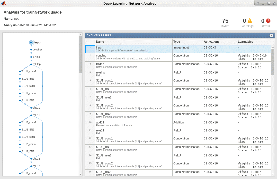
You can use analyzeNetwork to analyze the deep learning network architecture.

analyzeNetwork(net)

Load Data

Download the CIFAR-10 data set [1] by executing the code below. The data set contains 60,000 images. Each image is 32-by-32 in size and has three color channels (RGB). The size of the data set is 175 MB. Depending on your internet connection, the download process can take some time.

datadir = tempdir;
downloadCIFARData(datadir);

Prepare Data for Calibration and Validation

Load the CIFAR-10 training and test images as 4-D arrays. The training set contains 50,000 images and the test set contains 10,000 images. Use the CIFAR-10 test images for network validation.

[XTrain,YTrain,XValidation,YValidation] = loadCIFARData(datadir);

You can display a random sample of the training images using the following code.

figure;
idx = randperm(size(XTrain,4),20);
im = imtile(XTrain(:,:,:,idx),'ThumbnailSize',[96,96]);
imshow(im)

Create an augmentedImageDatastore object to use for calibration and validation. Use 200 random images for calibration and 50 random images for validation.

inputSize = net.Layers(1).InputSize;

augimdsTrain = augmentedImageDatastore(inputSize,XTrain,YTrain);
augimdsCalibration = shuffle(augimdsTrain).subset(1:200);

augimdsValidation = augmentedImageDatastore(inputSize,XValidation,YValidation);
augimdsValidation = shuffle(augimdsValidation).subset(1:50);

Quantize the Network for GPU Deployment Using the Deep Network Quantizer App

This example uses a GPU execution environment. To learn about the products required to quantize and deploy the deep learning network to a GPU environment, see Quantization Workflow Prerequisites (Deep Learning Toolbox).

In the MATLAB® Command Window, open the Deep Network Quantizer app.

deepNetworkQuantizer

Select New > Quantize a network. The app automatically verifies your execution environment.

In the dialog, select the execution environment and the network to quantize from the base workspace. For this example, select a GPU execution environment and the DAG network net.

In the Calibrate section of the toolstrip, under Calibration Data, select the augmentedImageDatastore object from the base workspace containing the calibration data augimdsCalibration.

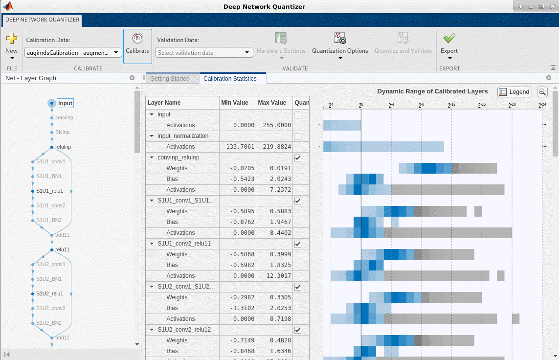
Click Calibrate.

Deep Network Quantizer uses the calibration data to exercise the network and collect range information for the learnable parameters in the network layers.

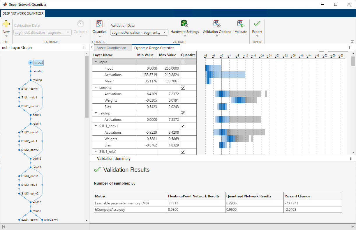
When the calibration is complete, the app displays a table containing the weights and biases in the convolution, as well as fully connected layers of the network and the dynamic ranges of the activations in all layers of the network with their minimum and maximum values during the calibration. To the right of the table, the app displays histograms of the dynamic ranges of the parameters. The gray regions of the histograms indicate data that cannot be represented by the quantized representation. For more information on how to interpret these histograms, see Quantization of Deep Neural Networks (Deep Learning Toolbox).

In the Quantize Layer column of the table, indicate whether to quantize the learnable parameters in the layer. Layers that are not convolution layers cannot be quantized, and therefore cannot be selected. Layers that are not quantized remain in single precision after quantization.

In the Validate section of the toolstrip, under Validation Data, select the augmentedImageDatastore object from the base workspace containing the validation data, augimdsValidation.

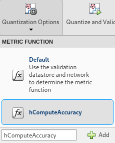
In the Validate section of the toolstrip, under Quantization Options, select the metric function to use for validation. The app determines a default metric function to use for validation based on the type of network that you quantize. You can also add additional custom metric functions to use for validation. For this example, enter the name of the custom metric function hComputeAccuracy. Select Add to add hComputeAccuracy to the list of metric functions available in the app. Select hComputeAccuracy as the metric function to use for validation. This custom metric function compares the predicted label to the ground truth and returns the top-1 accuracy. The custom metric function must be on the path.

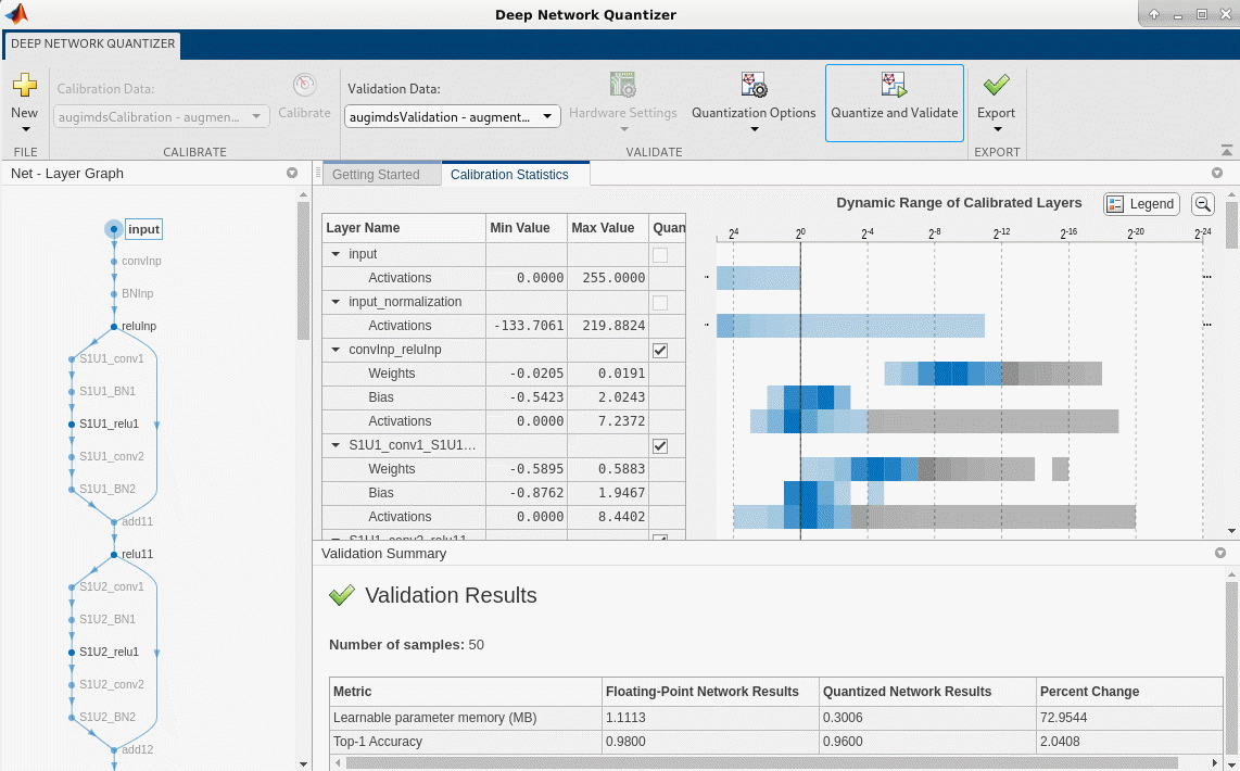
Click Quantize and Validate.

The app quantizes the network and displays a summary of the validation results. For this set of calibration and validation images, quantization of the network results in a 2% decrease in accuracy with a 73% reduction in learnable parameter memory for the set of 50 validation images.

After quantizing and validating the network, you can export the network or generate code. To export the network, select Export > Export Quantizer to create a dlquantizer object in the base workspace. To open the GPU Coder app and generate GPU code from the optimized neural network, select Export > Generate Code. To learn how to generate CUDA code for an optimized deep convolutional neural network using GPU Coder, see Generate INT8 Code for Deep Learning Networks.

Validate the Performance of the Network Using Multiple Metric Functions

You can use multiple metric functions to evaluate the performance of the network simultaneously by using the dlquantizer function.

To begin, load the pretrained network and data, and prepare the data for calibration and validation, as described above.

Create a dlquantizer object. Specify the network to quantize and the execution environment to use. Use the calibrate function to exercise the network with sample inputs from augimdsCalibration and collect range information.

dq = dlquantizer(net,'ExecutionEnvironment','GPU');
calResults = calibrate(dq,augimdsCalibration)

calResults=100×5 table
     Optimized Layer Name     Network Layer Name    Learnables / Activations    MinValue     MaxValue
    ______________________    __________________    ________________________    _________    ________

    {'convInp_Weights'   }      {'convInp'   }             "Weights"            -0.020545    0.01913 
    {'convInp_Bias'      }      {'convInp'   }             "Bias"                -0.54225     2.0243 
    {'S1U1_conv1_Weights'}      {'S1U1_conv1'}             "Weights"             -0.58949     0.5883 
    {'S1U1_conv1_Bias'   }      {'S1U1_conv1'}             "Bias"                -0.87623     1.9467 
    {'S1U1_conv2_Weights'}      {'S1U1_conv2'}             "Weights"             -0.58679    0.39988 
    {'S1U1_conv2_Bias'   }      {'S1U1_conv2'}             "Bias"                -0.59824     1.8325 
    {'S1U2_conv1_Weights'}      {'S1U2_conv1'}             "Weights"             -0.29821    0.33049 
    {'S1U2_conv1_Bias'   }      {'S1U2_conv1'}             "Bias"                 -1.3102     2.0253 
    {'S1U2_conv2_Weights'}      {'S1U2_conv2'}             "Weights"              -0.7149    0.48284 
    {'S1U2_conv2_Bias'   }      {'S1U2_conv2'}             "Bias"                -0.84685     1.6346 
    {'S1U3_conv1_Weights'}      {'S1U3_conv1'}             "Weights"             -0.16697    0.15356 
    {'S1U3_conv1_Bias'   }      {'S1U3_conv1'}             "Bias"                 -1.3796     2.1583 
    {'S1U3_conv2_Weights'}      {'S1U3_conv2'}             "Weights"             -0.47026    0.60147 
    {'S1U3_conv2_Bias'   }      {'S1U3_conv2'}             "Bias"                 -1.0089     1.5606 
    {'S2U1_conv1_Weights'}      {'S2U1_conv1'}             "Weights"             -0.14931    0.13792 
    {'S2U1_conv1_Bias'   }      {'S2U1_conv1'}             "Bias"                 -1.8735     2.4623 
      ⋮

Specify the metric functions in a dlquantizationOptions object. Use the validate function to quantize the learnable parameters in the convolution layers of the network and exercise the network. The validate function uses the metric functions defined in the dlquantizationOptions object to compare the results of the network before and after quantization. For this example, use the top-1 accuracy and top-5 accuracy metrics are used to evaluate the performance of the network.

dqOpts = dlquantizationOptions('Target','gpu', ...
    'MetricFcn',...
    {@(x)hComputeAccuracy(x,net,augimdsValidation), ...
    @(x)hComputeTop_5(x,net,augimdsValidation)});

validationResults = validate(dq,augimdsValidation,dqOpts)

validationResults = struct with fields:
       NumSamples: 50
    MetricResults: [1×2 struct]
       Statistics: [2×2 table]

Examine the MetricResults.Result field of the validation output to see the performance of the optimized network as measured by each metric function used.

validationResults.MetricResults.Result

ans=2×2 table
    NetworkImplementation    MetricOutput
    _____________________    ____________

     {'Floating-Point'}          0.98    
     {'Quantized'     }          0.96

ans=2×2 table
    NetworkImplementation    MetricOutput
    _____________________    ____________

     {'Floating-Point'}           1      
     {'Quantized'     }           1

validationResults.Statistics

ans=2×2 table
    NetworkImplementation    LearnableParameterMemory(bytes)
    _____________________    _______________________________

     {'Floating-Point'}                1.1113e+06           
     {'Quantized'     }                2.9865e+05

To visualize the calibration statistics, first save the dlquantizer object dq.

save('dlquantObj.mat','dq')

Then import the dlquantizer object dq in the Deep Network Quantizer app by selecting New > Import dlquantizer object.

Generate CUDA Code

Generate CUDA® code for an optimized deep convolutional neural network.

Create Entry-Point Function

Write an entry-point function in MATLAB® that:

Uses the coder.loadDeepLearningNetwork function to load a deep learning model and to construct and set up a CNN class. For more information, see Load Pretrained Networks for Code Generation.
Calls predict (Deep Learning Toolbox) to predict the responses.

type('mynet_predict.m');

function out = mynet_predict(netFile, im)
    persistent net; 
    if isempty(net)
        net = coder.loadDeepLearningNetwork(netFile);
    end
    out = net.predict(im);
end

A persistent object mynet loads the DAGNetwork object. The first call to the entry-point function constructs and sets up the persistent object. Subsequent calls to the function reuse the same object to call predict on inputs, avoiding reconstructing and reloading the network object.

Code Generation by Using `codegen`

To configure build settings such as the output file name, location, and type, you create coder configuration objects. To create the objects, use the coder.gpuConfig function. For example, when generating CUDA MEX using the codegen command, use cfg = coder.gpuConfig('mex').

To specify code generation parameters for cuDNN, set the DeepLearningConfig property to a coder.CuDNNConfig object that you create by using coder.DeepLearningConfig.

Specify the location of the MAT file containing the calibration data.

Specify the precision of the inference computations in supported layers by using the DataType property. For 8-bit integers, use 'int8'. Int8 precision requires a CUDA GPU with compute capability of 6.1, 6.3, or higher. Use the ComputeCapability property of the GPU code configuration object to set the appropriate compute capability value.

cfg = coder.gpuConfig('mex');
cfg.TargetLang = 'C++';
cfg.DeepLearningConfig = coder.DeepLearningConfig('cudnn');
cfg.DeepLearningConfig.DataType = 'int8';
cfg.DeepLearningConfig.CalibrationResultFile = 'dlquantObj.mat';
netFile = 'mynet.mat';
save(netFile,'net');

Run the codegen command. The codegen command generates CUDA code from the mynet_predict.m entry-point function.

codegen -config cfg mynet_predict -args {coder.Constant(netFile), ones(inputSize, 'single')} -report

When code generation is successful, you can view the resulting code generation report by clicking View Report in the MATLAB Command Window. The report is displayed in the Report Viewer window. If the code generator detects errors or warnings during code generation, the report describes the issues and provides links to the problematic MATLAB code. See Code Generation Reports.

References

[1] Krizhevsky, Alex. 2009. "Learning Multiple Layers of Features from Tiny Images." https://www.cs.toronto.edu/~kriz/learning-features-2009-TR.pdf

Quantize Residual Network Trained for Image Classification and Generate CUDA Code

Load Pretrained Network

Load Data

Prepare Data for Calibration and Validation

Quantize the Network for GPU Deployment Using the Deep Network Quantizer App

Validate the Performance of the Network Using Multiple Metric Functions

Generate CUDA Code

Create Entry-Point Function

Code Generation by Using `codegen`

References

See Also

Apps

Functions

Objects

Related Topics

Quantize Residual Network Trained for Image Classification and Generate CUDA Code

Load Pretrained Network

Load Data

Prepare Data for Calibration and Validation

Quantize the Network for GPU Deployment Using the Deep Network Quantizer App

Validate the Performance of the Network Using Multiple Metric Functions

Generate CUDA Code

Create Entry-Point Function

Code Generation by Using codegen

References

See Also

Apps

Functions

Objects

Related Topics

Code Generation by Using `codegen`