Compare Adaptive Pipelining and Improved Adaptive Pipelining on a Field-Oriented Control Design (Tech Preview)
R2026bNote
Improved adaptive pipelining is a tech preview in R2026b. The behavior, implementation, and interfaces might change before general release. Do not use the optimization in production designs.
To enable the improved adaptive pipelining optimization, run this command at the start of each MATLAB session:
matlab.internal.feature("GlobalAdaptivePipelining",1);To send feedback about improved adaptive pipelining, email the development team.
In this example, you compare the synthesis results from adaptive pipelining and improved
adaptive pipelining on a field-oriented control design. The
hdlcoderFocCurrentFixptHdl model is designed to run with clock-rate
pipelining enabled, so that HDL Coder can insert pipeline registers on the faster clock-rate
domain that the model creates from its oversampled input rates. This example targets the AMD
Zynq UltraScale+ MPSoC xczu9eg-ffvb1156-1-e device at a 100 MHz target frequency. Adaptive
pipelining combines manual InputPipeline values on the design under test
(DUT) subsystem with DistributedPipelining on the same subsystem, and can
require iterative tuning across code generation runs. Improved adaptive pipelining meets the
same target in a single code generation pass, with less hardware resource use.
Open Model
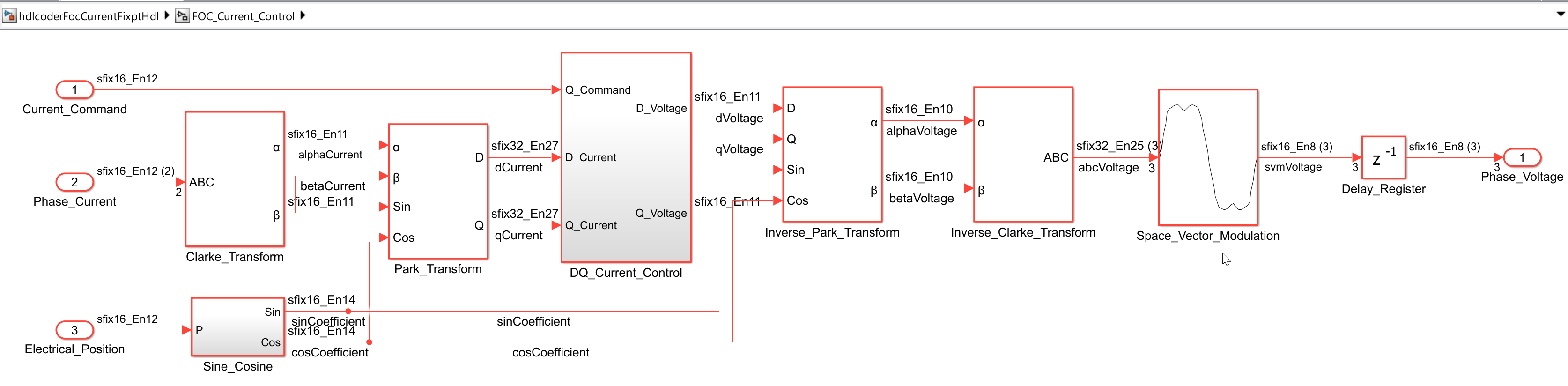
Open the hdlcoderFocCurrentFixptHdl example.
openExample("hdlcoder/FieldOrientedControlOfAPermanentMagnetSynchronousMachineExample");
model = "hdlcoderFocCurrentFixptHdl";
dut = "hdlcoderFocCurrentFixptHdl/FOC_Current_Control";
Enable and Run Adaptive Pipelining
Establish the adaptive pipelining result as the baseline you compare against. Configure the DUT and model:
Turn on adaptive pipelining and distributed pipelining on the DUT.
Add one input pipeline stage on the DUT so the input-pipeline setting matches the improved adaptive pipelining run and the comparison isolates the optimization.
Set the model to treat rates as hardware rates so pipelining places registers at the faster clock-rate domain.
Set
SubsystemReusetooffso the two PI current controllers insideDQ_Current_Controlsynthesize as independent hardware and each instance participates in pipelining decisions on its own.
matlab.internal.feature("GlobalAdaptivePipelining", 0);
hdlset_param(dut, "AdaptivePipelining",    "on");
hdlset_param(dut, "DistributedPipelining", "on");
hdlset_param(dut, "InputPipeline",         1);
hdlset_param(dut, "OutputPipeline",        0);

hdlset_param(model, ...
    "TargetLanguage",            "Verilog", ...
    "TargetFrequency",           100, ...
    "SynthesisTool",             "Xilinx Vivado", ...
    "SynthesisToolChipFamily",   "Zynq UltraScale+", ...
    "SynthesisToolDeviceName",   "xczu9eg", ...
    "SynthesisToolPackageName",  "ffvb1156", ...
    "SynthesisToolSpeedValue",   "-1", ...
    "CriticalPathEstimation",    "on", ...
    "TreatRatesAsHardwareRates", "on", ...
    "SubsystemReuse",            "off");
Generate HDL code for the DUT:
makehdl(dut);
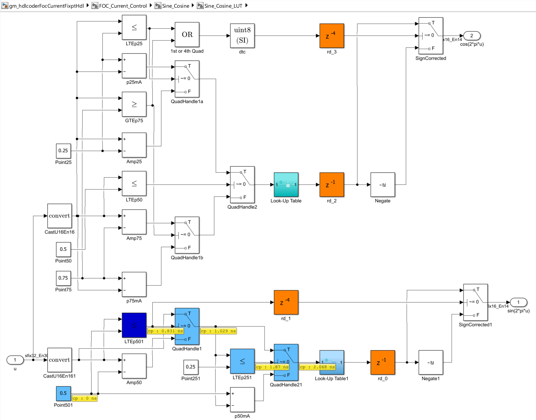
The critical path estimation (CPE) report lists the blocks along the estimated critical
path in propagation order. The cumulative propagation ends at the
Sine_Cosine subsystem output at 4.467 ns, which results in +5.533 ns of
estimated slack against the 10.000 ns budget.
| Stage | Block | Delay (ns) | Cumulative Propagation (ns) |
|---|---|---|---|
| 1 | Point501 (Sine_Cosine_LUT) | 0.000 | 0.000 |
| 2 | LTEp501 (Sine_Cosine_LUT) | 0.831 | 0.831 |
| 3 | QuadHandle1 (Sine_Cosine_LUT) | 0.198 | 1.029 |
| 4 | LTEp251 (Sine_Cosine_LUT) | 0.841 | 1.870 |
| 5 | QuadHandle21 (Sine_Cosine_LUT) | 0.198 | 2.068 |
| 6 | Look-Up Table1 (Sine_Cosine_LUT) | 2.399 | 4.467 |
| 7 | Sine_Cosine_LUT (subsystem output) | 0.000 | 4.467 |
| 8 | Sine_Cosine (subsystem output) | 0.000 | 4.467 |
This figure shows the Sine_Cosine_LUT subsystem interior from the
adaptive pipelining and distributed pipelining generated model.
Confirm the estimate by running synthesis. For more information on HDL code generation and FPGA synthesis from a Simulink model, see HDL Code Generation and FPGA Synthesis from Simulink Model. This run reaches an Fmax of 225.94 MHz, above the 100 MHz target, with a worst-negative slack of +5.574 ns.
Enable and Run Improved Adaptive Pipelining
Enable improved adaptive pipelining and re-run at the same 100 MHz target. Change the DUT optimization settings:
Enable improved adaptive pipelining and turn off distributed pipelining on the DUT.
Add one input pipeline stage on the DUT.
Enable critical path estimation to examine the paths that limit the achievable frequency.
matlab.internal.feature("GlobalAdaptivePipelining", 1);
hdlset_param(dut, "AdaptivePipelining",    "on");
hdlset_param(dut, "DistributedPipelining", "off");
hdlset_param(dut, "InputPipeline",         1);
hdlset_param(dut, "OutputPipeline",        0);

hdlset_param(model, ...
    "TargetLanguage",            "Verilog", ...
    "TargetFrequency",           100, ...
    "SynthesisTool",             "Xilinx Vivado", ...
    "SynthesisToolChipFamily",   "Zynq UltraScale+", ...
    "SynthesisToolDeviceName",   "xczu9eg", ...
    "SynthesisToolPackageName",  "ffvb1156", ...
    "SynthesisToolSpeedValue",   "-1", ...
    "CriticalPathEstimation",    "on", ...
    "TreatRatesAsHardwareRates", "on", ...
    "SubsystemReuse",            "off");
Generate HDL code for the DUT:
makehdl(dut);
Note
In R2026b, the adaptive pipelining report only reports multiplier-adjacent pipeline
registers. For this configuration, improved adaptive pipelining does not insert
multiplier-adjacent pipeline registers. The guide registers that the optimization places,
such as FOC_Current_Control/Sine_Cosine/Sine_Cosine_LUT/Negate_out1_guide
and FOC_Current_Control/cosCoefficient_guide, are sufficient to meet the
100 MHz target. As a result, the adaptive pipelining HTML report indicates that no pipeline
registers were inserted for the multipliers. An empty report does not mean improved adaptive
pipelining is inactive, the guide registers are the evidence that the optimization ran. To
see the full set of registers that improved adaptive pipelining inserted, open the generated
gm_hdlcoderFocCurrentFixptHdl.slx model, or search the generated
Verilog for processes with names ending in _guide_process. In other
designs, or at faster target frequencies, improved adaptive pipelining pipelines the
multipliers directly and the adaptive pipelining report indicates the inserted
stages.
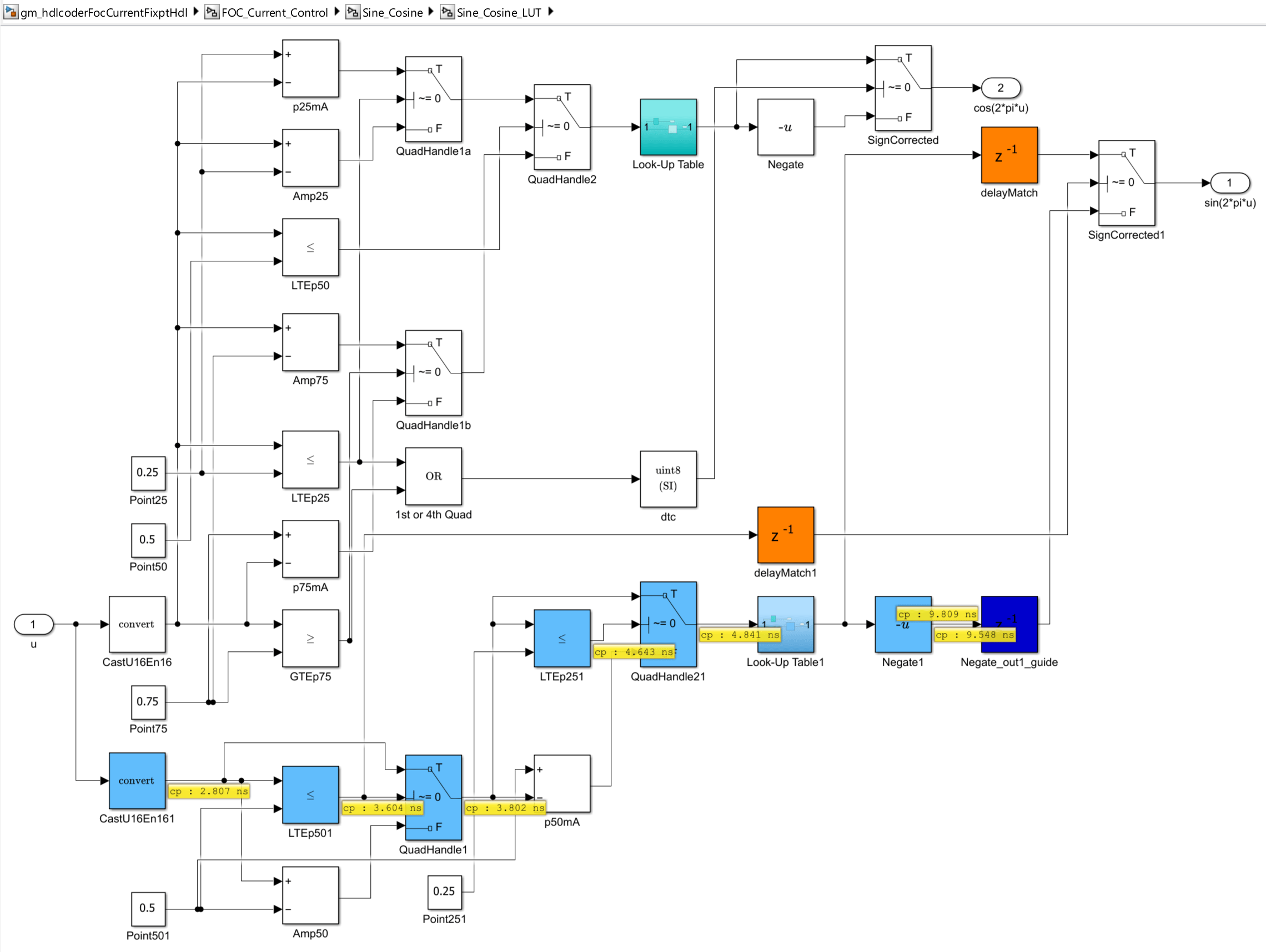
The critical path estimation (CPE) report lists the blocks along the estimated critical
path in propagation order. The cumulative propagation ends at the
Negate_out1_guide register at 9.809 ns, which results in +0.191 ns of
estimated slack against the 10.000 ns budget.
| Stage | Block | Delay (ns) | Cumulative Propagation (ns) |
|---|---|---|---|
| 1 | in_2_pipe_in_pipe (DUT input pipeline register) | 0.330 | 0.330 |
| 2 | Normalize_Position (Sine_Cosine) | 2.477 | 2.807 |
| 3 | CastU16En161 (Sine_Cosine_LUT) | 0.000 | 2.807 |
| 4 | LTEp501 (Sine_Cosine_LUT) | 0.797 | 3.604 |
| 5 | QuadHandle1 (Sine_Cosine_LUT) | 0.198 | 3.802 |
| 6 | LTEp251 (Sine_Cosine_LUT) | 0.841 | 4.643 |
| 7 | QuadHandle21 (Sine_Cosine_LUT) | 0.198 | 4.841 |
| 8 | Look-Up Table1 (Sine_Cosine_LUT) | 4.023 | 8.864 |
| 9 | Negate1 (Sine_Cosine_LUT) | 0.684 | 9.548 |
| 10 | Negate_out1_guide (Improved adaptive pipelining
register) | 0.261 | 9.809 |
This figure shows the Sine_Cosine_LUT subsystem interior from the
improved adaptive pipelining generated model.
Confirm the estimate by running synthesis. For more information on HDL code generation and FPGA synthesis from a Simulink model, see HDL Code Generation and FPGA Synthesis from Simulink Model. This run reaches an Fmax of 107.49 MHz, above the 100 MHz target, with a worst-negative slack of +0.697 ns.
Compare Synthesis Results
Compare the post-implementation timing and resource reports for the two configurations. This table lists the synthesis data.
| Approach | Latency | CPE (ns) | Fmax (MHz) | LUT | FF | DSP | BRAM |
|---|---|---|---|---|---|---|---|
| Adaptive pipelining and distributed pipelining | 0 cycles | 4.467 | 225.94 | 1478 | 1254 | 21 | 1 |
| Improved adaptive pipelining | 0 cycles | 9.809 | 107.49 | 1201 | 505 | 21 | 1 |
Improved adaptive pipelining produces a smaller implementation than the adaptive
pipelining approach and meets the 100 MHz target. Improved adaptive pipelining places guide
registers such as
FOC_Current_Control/Sine_Cosine/Sine_Cosine_LUT/Negate_out1_guide and
FOC_Current_Control/cosCoefficient_guide at the boundaries it selects,
which reduces the estimated critical path to 9.809 ns and closes 100 MHz timing with WNS
+0.697 ns at 107.49 MHz. The adaptive and distributed pipelining approach reaches a higher
Fmax, 225.94 MHz, but improved adaptive pipelining uses about 60% fewer flip-flops and about
19% fewer LUTs. For applications where the 100 MHz target is the design requirement, improved
adaptive pipelining reaches that target in a single code generation pass and generates a
leaner implementation.
Because you set TreatRatesAsHardwareRates to on, the
Latency column reports only the DUT output-port compensation delay; the actual internal
pipeline depth appears in the generated Verilog. For example, the guide register that improved
adaptive pipelining inserts at the LUT negate output appears in
hdlsrc/hdlcoderFocCurrentFixptHdl/Sine_Cosine_LUT.v:
always @(posedge clk)
  begin : Negate_out1_guide_process
    if (reset == 1'b1) begin
      Negate_out1_1 <= 16'sb0000000000000000;
    end
    else begin
      if (enb) begin
        Negate_out1_1 <= Negate_out1;
      end
    end
  end
