Identify Linear Models Using System Identification App

Introduction

Objectives

Estimate and validate linear models from single-input/single-output (SISO) data to find the one that best describes the system dynamics.

After completing this tutorial, you will be able to accomplish the following tasks using the System Identification app:

Import data arrays from the MATLAB^® workspace into the app.
Plot the data.
Process data by removing offsets from the input and output signals.
Estimate, validate, and compare linear models.
Export models to the MATLAB workspace.

Note

The tutorial uses time-domain data to demonstrate how you can estimate linear models. The same workflow applies to fitting frequency-domain data.

This tutorial is based on the example in section 17.3 of System Identification: Theory for the User, Second Edition, by Lennart Ljung, Prentice Hall PTR, 1999.

Data Description

This tutorial uses the data file dryer2.mat, which contains single-input/single-output (SISO) time-domain data from Feedback Process Trainer PT326. The input and output signals each contain 1000 data samples.

This system heats the air at the inlet using a mesh of resistor wire, similar to a hair dryer. The input is the power supplied to the resistor wires, and the output is the air temperature at the outlet.

Preparing Data for System Identification

Loading Data into the MATLAB Workspace

Load the data in dryer2.mat by typing the following command in the MATLAB Command Window:

load dryer2

This command loads the data into the MATLAB workspace as two column vectors, u2 and y2, respectively. The variable u2 is the input data and y2 is the output data.

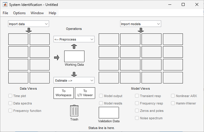
Opening the System Identification App

To open the System Identification app, type the following command in the MATLAB Command Window:

systemIdentification

The default session name, Untitled, appears in the title bar.

System Identification app main screen. The Import data area is on the left and includes Data Views selections at the bottom. The Operations area is to the right of the Import data area. The Import models area is on the right and includes Model Views selections at the bottom.

Importing Data Arrays into the System Identification App

You can import the single-input/single-output (SISO) data from a sample data file dryer2.mat into the app from the MATLAB workspace.

You must have already loaded the sample data into MATLAB, as described in Loading Data into the MATLAB Workspace, and opened the System Identification app, as described in Opening the System Identification App.

If you have not performed these steps, click here to complete them.

To import data arrays into the System Identification app:

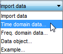
Select Import data > Time domain data. This action opens the Import Data dialog box.
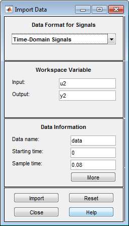
In the Import Data dialog box, specify the following options:
- Input — Enter u2 as the name of the input variable.
- Output — Enter y2 as the name of the output variable.
- Data name — Change the default name to data. This name labels the data in the System Identification app after the import operation is completed.
- Starting time — Enter 0 as the starting time. This value designates the starting value of the time axis on time plots.
- Sample Time — Enter 0.08 as the time between successive samples in seconds. This value is the actual sample time in the experiment.
The Import Data dialog box now resembles the following figure.
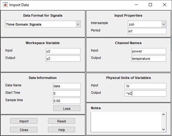
In the Data Information area, click More to expand the dialog box and specify the following options:
Input Properties
- Intersample — Accept the default zoh (zero-order hold) to indicate that the input signal was piecewise-constant between samples during data acquisition. This setting specifies the behavior of the input signals between samples when you transform the resulting models between discrete-time and continuous-time representations.
- Period — Accept the default inf to specify a nonperiodic input.
  Note
  For a periodic input, enter the whole number of periods of the input signal in your experiment.
Channel Names
- Input — Enter power.
  Tip
  Naming channels helps you to identify data in plots. For multivariable input and output signals, you can specify the names of individual Input and Output channels, separated by commas.
- Output — Enter temperature.
Physical Units of Variables
- Input — Enter W for power units.
  Tip
  When you have multiple inputs and outputs, enter a comma-separated list of Input and Output units corresponding to each channel.
- Output — Enter ^oC for temperature units.
Notes — Enter comments about the experiment or the data. For example, you might enter the experiment name, date, and a description of experimental conditions. When you estimate models from this data, these models inherit your notes.
The expanded Import Data dialog box now resembles the following figure.
Click Import to add the data to the System Identification app. The app displays an icon to represent the data.
Click Close to close the Import Data dialog box.

Plotting and Processing Data

In this portion of the tutorial, you evaluate the data and process it for system identification. You learn how to:

Plot the data.
Remove offsets from the data by subtracting the mean values of the input and the output.
Split the data into two parts to use one part model estimation and the other part for model validation.

The reason you subtract the mean values from each signal is because, typically, you build linear models that describe the responses for deviations from a physical equilibrium. With steady-state data, it is reasonable to assume that the mean levels of the signals correspond to such an equilibrium. Thus, you can seek models around zero without modeling the absolute equilibrium levels in physical units.

You must have already imported data into the System Identification app, as described in Importing Data Arrays into the System Identification App.

If you have not performed this step, click here to complete it.

To plot and process the data:

Select the Time plot check box to open the Time Plot. If the plot window is empty, click the data icon in the System Identification app.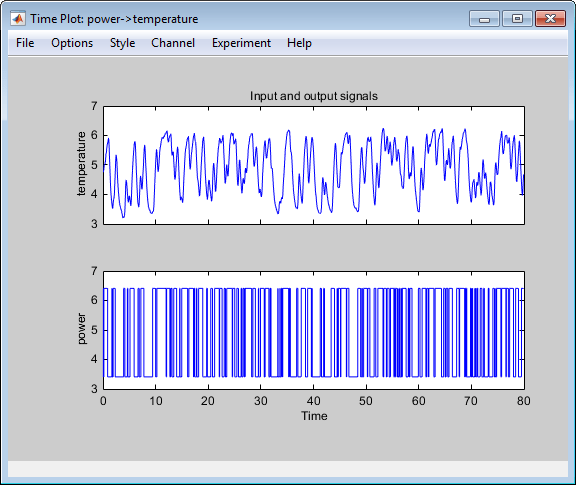
The top axes show the output data (temperature), and the bottom axes show the input data (power). Both the input and the output data have nonzero mean values.
Subtract the mean input value from the input data and the mean output value from the output data. In the System Identification app, select <--Preprocess > Remove means.
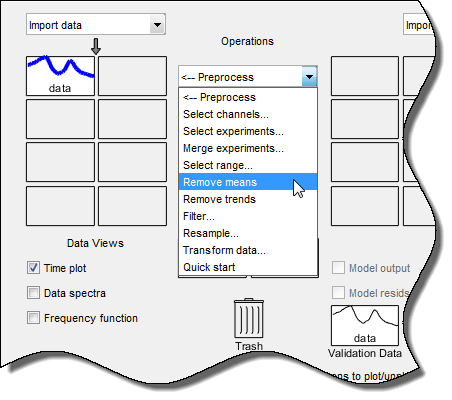
This action adds a new data set to the System Identification app with the default name datad (the suffix d means detrend), and updates the Time Plot window to display both the original and the detrended data. The detrended data has a zero mean value.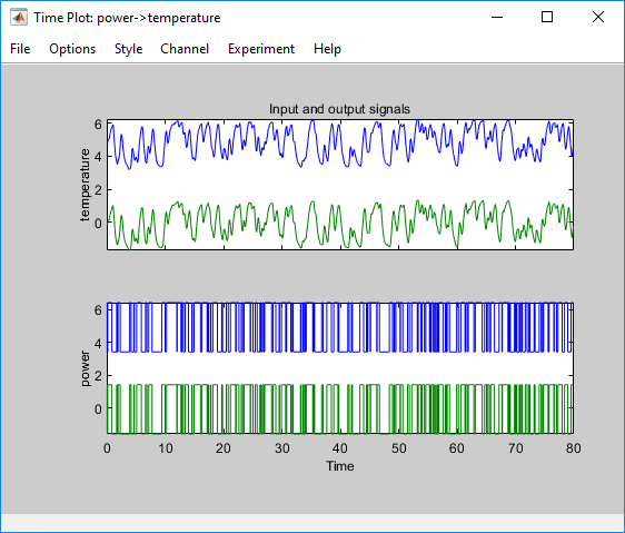
Specify the detrended data to be used for estimating models. Drag the data set datad to the Working Data rectangle.
Alternatively, right-click the datad icon to open the Data/model Info dialog box.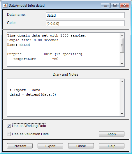
Select the Use as Working Data check-box. Click Apply and then Close. This action adds datad to the Working Data rectangle.
Split the data into two parts and specify the first part for model estimation, and the second part for model validation.
1. Select <--Preprocess > Select range to open the Select Range window.
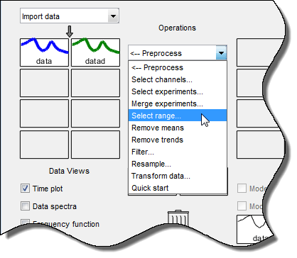
2. In the Select Range window, create a data set containing the first 500 samples. In the Samples field, specify 1 500.
  Tip
  You can also select data samples using the mouse by clicking and dragging a rectangular region on the plot. If you select samples on the input-channel axes, the corresponding region is also selected on the output-channel axes.
3. In the Data name field, type the name data_est.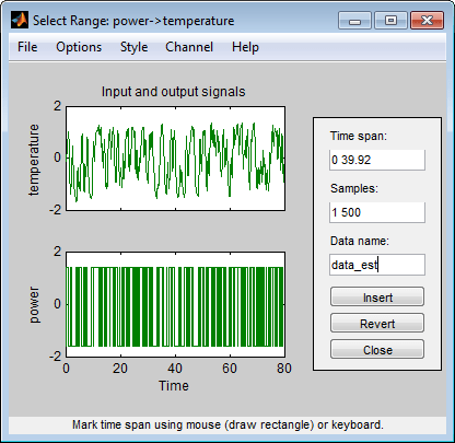
4. Click Insert to add this new data set to the System Identification app to be used for model estimation.
5. Repeat this process to create a second data set containing a subset of the data to use for validation. In the Select Range window, specify the last 500 samples in the Samples field. Type the name data_val in the Data name field. Click Insert to add this new data set to the System Identification app.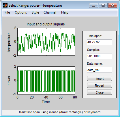
6. Click Close to close the Select Range window.
In the System Identification app, drag and drop data_est to the Working Data rectangle, and drag and drop data_val to the Validation Data rectangle.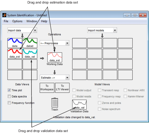
To get information about a data set, right-click its icon. For example, right-click data_est to open the Data/model Info dialog box.
You can also change certain values in the Data/model Info dialog box, including:
- Changing the name of the data set in the Data name field.
- Changing the color of the data icon in the Color field. You specify colors using RGB values (relative amounts of red, green, and blue). Each value is between 0 and 1. For example, [1,0,0] indicates that only red is present, and no green and blue are mixed into the overall color.
- Viewing or editing the commands executed on this data set in the Diary and Notes area. This area contains the command-line equivalent to the processing you performed using the System Identification app. For example, as shown in the Data/model Info: estimate window, the data_est data set is a result of importing the data, detrending the mean values, and selecting the first 500 samples of the data.
  % Import data datad = detrend(data,0) data_est = datad([1:500])
  For more information about these and other toolbox commands, see the corresponding reference pages.

The Data/model Info dialog box also displays the total number of samples, the sample time, and the output and input channel names and units. This information is not editable.

Tip

As an alternative shortcut, you can select Preprocess > Quick start from the System Identification app to perform all of the data processing steps in this tutorial.

Learn More. For information about supported data processing operations, such as resampling and filtering the data, see Preprocess Data.

Saving the Session

After you process the data, as described in Plotting and Processing Data, you can delete any data sets in the window that you do not need for estimation and validation, and save your session. You can open this session later and use it as a starting point for model estimation and validation without repeating these preparatory steps.

You must have already processed the data into the System Identification app, as described in Plotting and Processing Data.

To delete specific data sets from a session and save the session:

In the System Identification app:
1. Drag and drop the data data set into Trash.
2. Drag and drop the datad data set into Trash.
Alternatively, you can press the Delete key on your keyboard to move the data sets to Trash.
Note
Moving items to the Trash does not delete them. To permanently delete items, select Options > Empty trash.
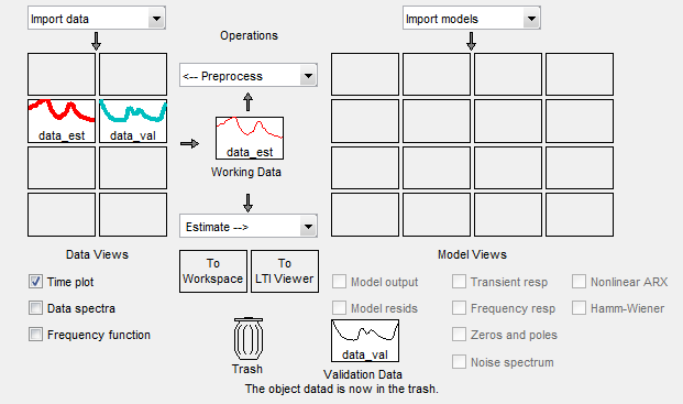
The following figure shows the System Identification app after moving the items to Trash.
Drag and drop the data_est and data_val data sets to fill the empty rectangles, as shown in the following figure.
Select File > Save session as to open the Save Session dialog box, and browse to the folder where you want to save the session file.
In the File name field, type the name of the session dryer2_processed_data, and click Save. The resulting file has a .sid extension.

Tip

You can open a saved session when starting the System Identification app by typing the following command at the MATLAB prompt:

systemIdentification('dryer2_processed_data')

For more information about managing sessions, see Starting and Managing Sessions.

Estimating Linear Models Using Quick Start

How to Estimate Linear Models Using Quick Start

You can use the Quick Start feature in the System Identification app to estimate linear models. Quick Start might produce the final linear models you decide to use, or provide you with information required to configure the estimation of accurate parametric models, such as time constants, input delays, and resonant frequencies.

You must have already processed the data for estimation, as described in Plotting and Processing Data.

If you have not performed this step, click here to complete it.

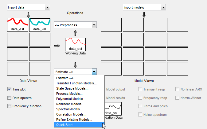
In the System Identification app, select Estimate > Quick Start.

This action generates plots of step response, frequency-response, and the output of state-space and polynomial models. For more information about these plots, see Validating the Quick Start Models.

Quick start is selected in the drop-down list for Estimate in the Operations area

Types of Quick Start Linear Models

Quick Start estimates the following four types of models and adds the following to the System Identification app with default names:

imp — Step response over a period of time using the impulseest algorithm.
spad — Frequency response over a range of frequencies using the spa algorithm. The frequency response is the Fourier transform of the impulse response of a linear system.
By default, the model is evaluated at 128 frequency values, ranging from 0 to the Nyquist frequency.
arxqs — Fourth-order autoregressive (ARX) model using the arx algorithm.
This model is parametric and has the following structure:
$\begin{array}{l} y (t) + a_{1} y (t - 1) + \dots + a_{n a} y (t - n_{a}) = \\ b_{1} u (t - n_{k}) + \dots + b_{n b} u (t - n_{k} - n_{b} + 1) + e (t) \end{array}$
y(t) represents the output at time t, u(t) represents the input at time t, n_a is the number of poles, n_b is the number of b parameters (equal to the number of zeros plus 1), n_k is the number of samples before the input affects output of the system (called the delay or dead time of the model), and e(t) is the white-noise disturbance. System Identification Toolbox™ software estimates the parameters $a_{1} \dots a_{n}$ and $b_{1} \dots b_{n}$ using the input and output data from the estimation data set.
In arxqs, n_a=n_b=4, and n_k is estimated from the step response model imp.
n4s3 — State-space model calculated using n4sid. The algorithm automatically selects the model order (in this case, 3).
This model is parametric and has the following structure:
$\begin{array}{l} \frac{d x}{d t} = A x (t) + B u (t) + K e (t) \\ y (t) = C x (t) + D u (t) + e (t) \end{array}$
y(t) represents the output at time t, u(t) represents the input at time t, x is the state vector, and e(t) is the white-noise disturbance. The System Identification Toolbox product estimates the state-space matrices A, B, C, D, and K.

Note

The Quick Start option does not create a transfer function model or a process model which can also be good starting model types.

Validating the Quick Start Models

Quick Start generates the following plots during model estimation to help you validate the quality of the models:

Step-response plot
Frequency-response plot
Model-output plot

You must have already estimated models using Quick Start to generate these plots, as described in How to Estimate Linear Models Using Quick Start.

If you have not performed this step, click here to complete it.

Step-Response Plot. The following step-response plot shows agreement among the different model structures and the measured data, which means that all of these structures have similar dynamics.

Tip

If you closed the plot window, select the Transient resp check box to reopen this window. If the plot is empty, click the model icons in the System Identification app window to display the models on the plot.

Step Response for imp, arxqs, and n4s3

Tip

You can use the step-response plot to estimate the dead time of linear systems. For example, the previous step-response plot shows a time delay of about 0.25 s before the system responds to the input. This response delay, or dead time, is approximately equal to about three samples because the sample time is 0.08 s for this data set.

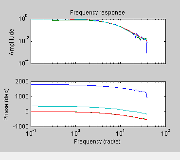
Frequency-Response Plot. The following frequency-response plot shows agreement among the different model structures and the measured data, which means that all of these structures have similar dynamics.

Tip

If you closed this plot window, select the Frequency resp check box to reopen this window. If the plot is empty, click the model icons in the System Identification app window to display the models on the plot.

Frequency Response for Models imp, spad, arxqs, and n4s3

Model-Output Plot. The Model Output window shows agreement among the different model structures and the measured output in the validation data.

Tip

If you closed the Model Output window, select the Model output check box to reopen this window. If the plot is empty, click the model icons in the System Identification app window to display the models on the plot.

Measured Output and Model Output for Models imp, arxqs, and n4s3

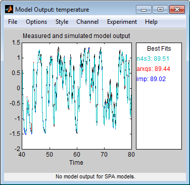
The model-output plot shows the model response to the input in the validation data. The fit values for each model are summarized in the Best Fits area of the Model Output window. The models in the Best Fits list are ordered from best at the top to worst at the bottom. The fit between the two curves is computed such that 100 means a perfect fit, and 0 indicates a poor fit (that is, the model output has the same fit to the measured output as the mean of the measured output).

In this example, the output of the models matches the validation data output, which indicates that the models seem to capture the main system dynamics and that linear modeling is sufficient.

Tip

To compare predicted model output instead of simulated output, select this option from the Options menu in the Model Output window.

Estimating Linear Models

Strategy for Estimating Accurate Models

The linear models you estimated in Estimating Linear Models Using Quick Start showed that a linear model sufficiently represents the dynamics of the system.

In this portion of the tutorial, you get accurate parametric models by performing the following tasks:

Identifying initial model orders and delays from your data using a simple, polynomial model structure (ARX).
Exploring more complex model structures with orders and delays close to the initial values you found.

The resulting models are discrete-time models.

Estimating Possible Model Orders

To identify black-box models, you must specify the model order. However, how can you tell what model orders to specify for your black-box models? To answer this question, you can estimate simple polynomial (ARX) models for a range of orders and delays and compare the performance of these models. You choose the orders and delays that correspond to the best model fit as an initial guess for more accurate modeling using various model structures such as transfer function and state-space models.

About ARX Models. For a single-input/single-output system (SISO), the ARX model structure is:

$\begin{array}{l} y (t) + a_{1} y (t - 1) + \dots + a_{n a} y (t - n_{a}) = \\ b_{1} u (t - n_{k}) + \dots + b_{n b} u (t - n_{k} - n_{b} + 1) + e (t) \end{array}$

y(t) represents the output at time t, u(t) represents the input at time t, n_a is the number of poles, n_b is the number of zeros plus 1, n_k is the input delay—the number of samples before the input affects the system output (called delay or dead time of the model), and e(t) is the white-noise disturbance.

You specify the model orders n_a, n_b, and n_k to estimate ARX models. The System Identification Toolbox product estimates the parameters $a_{1} \dots a_{n}$ and $b_{1} \dots b_{n}$ from the data.

How to Estimate Model Orders

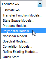
In the System Identification app, select Estimate > Polynomial Models to open the Polynomial Models dialog box.
From the Structure list, select ARX: [na nb nk]. By default, this is already selected.
Edit the Orders field to try all combinations of poles, zeros, and delays, where each value is from 1 to 10:
[1:10 1:10 1:10]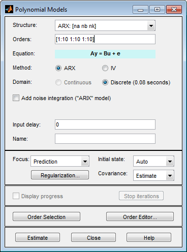
Click Estimate to open the ARX Model Structure Selection window, which displays the model performance for each combination of model parameters.
You use this plot to select the best-fit model.
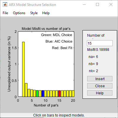
- The horizontal axis is the total number of parameters — n_a + n_b.
- The vertical axis, called Unexplained output variance (in %), is the portion of the output not explained by the model—the ARX model prediction error for the number of parameters shown on the horizontal axis.
  The prediction error is the sum of the squares of the differences between the validation data output and the model one-step-ahead predicted output.
- n_k is the delay.
Three rectangles are highlighted on the plot in green, blue, and red. Each color indicates a type of best-fit criterion, as follows:
- Red — Best fit minimizes the sum of the squares of the difference between the validation data output and the model output. This rectangle indicates the overall best fit.
- Green — Best fit minimizes Rissanen MDL criterion.
- Blue — Best fit minimizes Akaike AIC criterion.
In this tutorial, the Unexplained output variance (in %) value remains approximately constant for the combined number of parameters from 4 to 20. Such constancy indicates that model performance does not improve at higher orders. Thus, low-order models might fit the data equally well.
Note
When you use the same data set for estimation and validation, use the MDL and AIC criteria to select model orders. These criteria compensate for overfitting that results from using too many parameters. For more information about these criteria, see the selstruc reference page.
In the ARX Model Structure Selection window, click the red bar (corresponding to 15 on the horizontal axis), and click Insert. This selection inserts n_a=6, n_b=9, and n_k=2 into the Polynomial Models dialog box and performs the estimation.
This action adds the model arx692 to the System Identification app and updates the plots to include the response of the model.
Note
The default name of the parametric model contains the model type and the number of poles, zeros, and delays. For example, arx692 is an ARX model with n_a=6, n_b=9, and a delay of two samples.
In the ARX Model Structure Selection window, click the third bar corresponding to 4 parameters on the horizontal axis (the lowest order that still gives a good fit), and click Insert.
- This selection inserts n_a=2, n_b=2, and n_k=3 (a delay of three samples) into the Polynomial Models dialog box and performs the estimation.
- The model arx223 is added to the System Identification app and the plots are updated to include its response and output.
Click Close to close the ARX Model Structure Selection window.
Click Close to close the Polynomial Models dialog box.

Identifying Transfer Function Models

By estimating ARX models for different order combinations, as described in Estimating Possible Model Orders, you identified the number of poles, zeros, and delays that provide a good starting point for systematically exploring different models.

The overall best fit for this system corresponds to a model with six poles, nine zeros, and a delay of two samples. It also showed that a low-order model with n_a = 2 (two poles), n_b = 2 (one zero), and n_k = 3 (input-output delay) also provides a good fit. Thus, you should explore model orders close to these values.

In this portion of the tutorial, you estimate a transfer function model.

About Transfer Function Models. The general transfer function model structure is:

$Y (s) = \frac{n u m (s)}{d e n (s)} U (s) + E (s)$

Y(s), U(s) and E(s) represent the Laplace transforms of the output, input and error, respectively. num(s) and den(s) represent the numerator and denominator polynomials that define the relationship between the input and the output. The roots of the denominator polynomial are referred to as the model poles. The roots of the numerator polynomial are referred to as the model zeros.

You must specify the number of poles and zeros to estimate a transfer function model. The System Identification Toolbox product estimates the numerator and denominator polynomials, and input/output delays from the data.

The transfer function model structure is a good choice for quick estimation because it requires that you specify only 2 parameters to get started: np is the number of poles and nz is the number of zeros.

How to Estimate Transfer Function Models

In the System Identification app, select Estimate > Transfer Function Models to open the Transfer Functions dialog box.
In the Estimate Transfer Functions dialog box, specify the following options:
- Number of poles — Leave the default value 2 to specify a second order function, for two poles.
- Number of zeros — Leave the default value 1.
- Continuous-time — Leave this checked.
Click Delay to expand the input/output delay specification area.
By estimating ARX models for different order combinations, as described in Estimating Possible Model Orders, you identified a 3 sample delay (nk = 3). This delay translates to a continuous-time delay of (nk-1)*Ts, which is equal to 0.16 seconds.
Specify Delay as 0.16 seconds. Leave Fixed checked.
Use the default Estimation Options. By default, the app assigns the name tf1 to the model. The dialog box should look like this.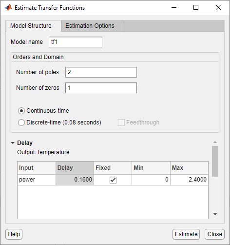
Click Estimate to add a transfer function model called tf1 to the System Identification app. You can view the output of the estimation of the transfer function model in comparison with the estimations of other models, in the Model output window.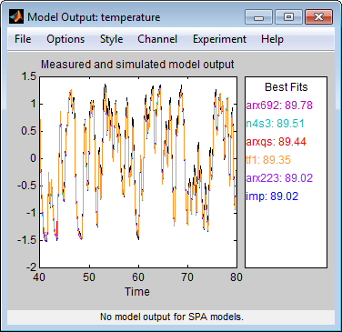
Tip
If you closed the Model Output window, you can regenerate it by selecting the Model output check box in the System Identification app. If the new model does not appear on the plot, click the model icon in the System Identification app to make the model active.
Click Close to close the Transfer Functions dialog box.

Learn More. To learn more about identifying transfer function models, see Transfer Function Models.

Identifying State-Space Models

The overall best fit for this system corresponds to a model with six poles, nine zeros, and a delay of two samples. It also showed that a low-order model with n_a=2 (two poles), n_b=2 (one zero), and n_k=3 (input-output delay) also provides a good fit. Thus, you should explore model orders close to these values.

In this portion of the tutorial, you estimate a state-space model.

About State-Space Models. The general state-space model structure (innovation form) is:

$\begin{array}{l} \frac{d x}{d t} = A x (t) + B u (t) + K e (t) \\ y (t) = C x (t) + D u (t) + e (t) \end{array}$

y(t) represents the output at time t, u(t) represents the input at time t, x(t) is the state vector at time t, and e(t) is the white-noise disturbance.

You must specify a single integer as the model order (dimension of the state vector) to estimate a state-space model. The System Identification Toolbox product estimates the state-space matrices A, B, C, D, and K from the data.

The state-space model structure is a good choice for quick estimation because it requires that you specify only the number of states (which equals the number of poles). You can optionally also specify the delays and feedthrough behavior.

How to Estimate State-Space Models

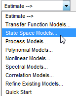
In the System Identification app, select Estimate > State Space Models to open the State Space Models dialog box.
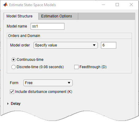
In the Specify value field of the Model Structure tab, specify the model order. Type 6 to create a sixth-order state-space model.
This choice is based on the fact that the best-fit ARX model has six poles.
Tip
Although this tutorial estimates a sixth-order state-space model, you might want to explore whether a lower-order model adequately represents the system dynamics.
The dialog box should look like this:
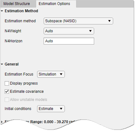
Select the Estimation Options tab to display additional options.
Change Estimation Focus to Simulation to optimize the model to use for output simulation.
The State Space Models dialog box looks like the following figure.
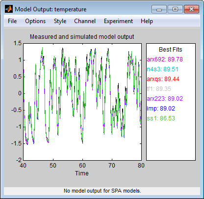
Click Estimate to add a state-space model called ss1 to the System Identification app.
You can view the output of the estimation of the state-space model in comparison with the estimations of other models, in the Model output window.
Tip
If you closed the Model Output window, you can regenerate it by selecting the Model output check box in the System Identification app. If the new model does not appear on the plot, click the model icon in the System Identification app to make the model active.
Click Close to close the State Space Models dialog box.

Learn More. To learn more about identifying state-space models, see State-Space Models.

Identifying ARMAX Models

The overall best fit for this system corresponds to a model with six poles, nine zeros, and a delay of two samples. It also showed that a low-order model with n_a=2 (two poles), n_b=2 (one zero), and n_k=3 also provides a good fit. Thus, you should explore model orders close to these values.

In this portion of the tutorial, you estimate an ARMAX input-output polynomial model.

About ARMAX Models. For a single-input/single-output system (SISO), the ARMAX polynomial model structure is:

$\begin{array}{l} y (t) + a_{1} y (t - 1) + \dots + a_{n a} y (t - n_{a}) = \\ b_{1} u (t - n_{k}) + \dots + b_{n b} u (t - n_{k} - n_{b} + 1) + \\ e (t) + c_{1} e (t - 1) + \dots + c_{n c} e (t - n_{c}) \end{array}$

y(t) represents the output at time t, u(t) represents the input at time t, n_a is the number of poles for the dynamic model, n_b is the number of zeros plus 1, n_c is the number of poles for the disturbance model, n_k is the number of samples before the input affects output of the system (called the delay or dead time of the model), and e(t) is the white-noise disturbance.

Note

The ARMAX model is more flexible than the ARX model because the ARMAX structure contains an extra polynomial to model the additive disturbance.

You must specify the model orders to estimate ARMAX models. The System Identification Toolbox product estimates the model parameters $a_{1} \dots a_{n}$ , $b_{1} \dots b_{n}$ , and $c_{1} \dots c_{n}$ from the data.

How to Estimate ARMAX Models

In the System Identification app, select Estimate > Polynomial Models to open the Polynomial Models dialog box.
From the Structure list, select ARMAX: [na nb nc nk] to estimate an ARMAX model.
In the Orders field, set the orders na, nb, nc, and nk to the following values:
[2 2 2 2]
The app assigns the name to the model amx2222, by default, visible in the Name field.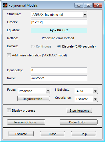
Click Estimate to add the ARMAX model to the System Identification app.
Repeat steps 3 and 4 using higher Orders 3 3 2 2. These orders result in a model that fits the data almost as well as the higher order ARX model arx692.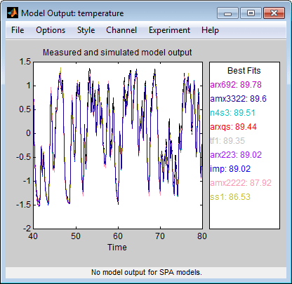
Tip
If you closed the Model Output window, you can regenerate it by selecting the Model output check box in the System Identification app. If the new model does not appear on the plot, click the model icon in the System Identification app to make the model active.
Click Close to close the Polynomial Models dialog box.

Learn More. To learn more about identifying input-output polynomial models, such as ARMAX, see Input-Output Polynomial Models.

Choosing the Best Model

You can compare models to choose the model with the best performance.

You must have already estimated the models, as described in Estimating Linear Models.

If you have not performed this step, click here to complete it.

Summary of Models. The following figure shows the System Identification app, which includes all the estimated models in Estimating Linear Models.

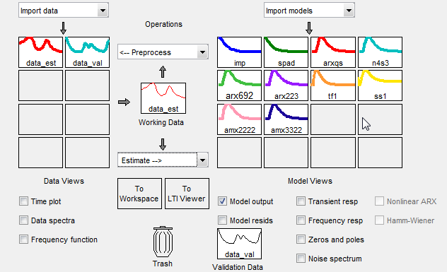
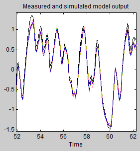
Examining the Model Output. Examine the model output plot to see how well the model output matches the measured output in the validation data set. A good model is the simplest model that best describes the dynamics and successfully simulates or predicts the output for different inputs. Models are listed by name in the Best Fits area of the Model Output plot. Note that one of the simpler models, amx3322, produced a similar fit as the highest-order model you created, arx692.

Tip

If you closed the Model Output window, you can regenerate it by selecting the Model output check box in the System Identification app. If the new model does not appear on the plot, click the model icon in the System Identification app to make the model active.

To validate your models using a different data set, you can drag and drop this data set into the Validation Data rectangle in the System Identification app. If you transform validation data into the frequency domain, the Model Output plot updates to show the model comparison in the frequency domain.

To get a closer look at how well these models fit the data, magnify a portion of the plot by clicking and dragging a rectangle around the region of interest, as shown in the following figure.

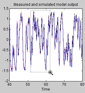
Releasing the mouse magnifies this region and shows that the output of all models matches the validation data well.

Viewing Model Parameters

Viewing Model Parameter Values

You can view the numerical parameter values for each estimated model.

You must have already estimated the models, as described in Estimating Linear Models.

If you have not performed this step, click here to complete it.

To view the parameter values of the model amx3322, right-click the model icon in the System Identification app. The Data/model Info dialog box opens.

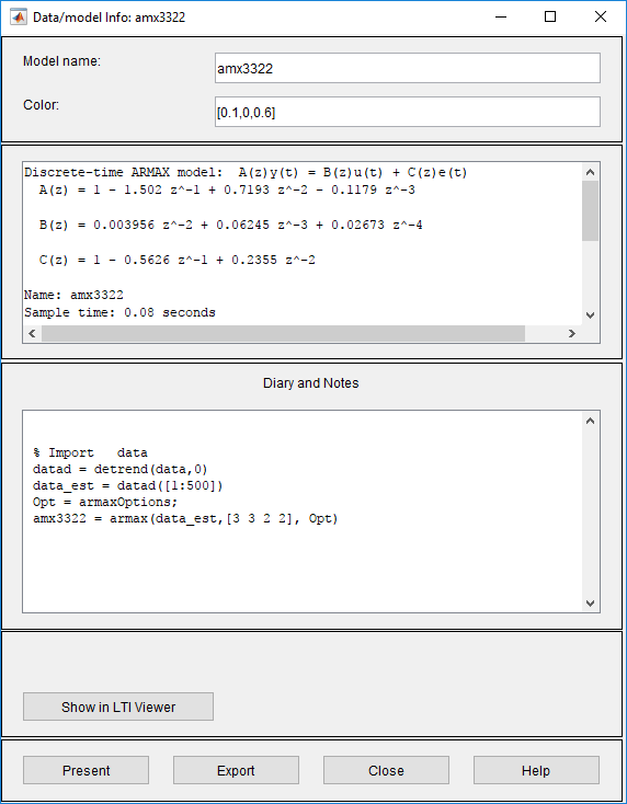
The noneditable area of the Data/model Info dialog box lists the parameter values correspond to the following difference equation for your system:

$\begin{array}{l} y (t) - 1.502 y (t - 1) + 0.7193 y (t - 2) - 0.1179 y (t - 3) = \\ 0.003956 u (t - 2) + 0.06245 u (t - 3) + 0.02673 u (t - 4) + e (t) - 0.5626 e (t - 1) + 0.2355 e (t - 2) \end{array}$

Note

The coefficient of u(t-2) is not significantly different from zero. This lack of difference explains why delay values of both 2 and 3 give good results.

Parameter values appear in the following format:

$\begin{array}{l} A (z) = 1 + a_{1} z^{- 1} + \dots + a_{n a} z^{- n a} \\ B (z) = b_{1} z^{- n k} + \dots + b_{n b} z^{- n b - n k + 1} \\ C (z) = 1 + c_{1} z^{- 1} + \dots + c_{n c} z^{- n c} \end{array}$

The parameters appear in the ARMAX model structure, as follows:

$A (q) y (t) = B (q) u (t) + C (q) e (t)$

which corresponds to this general difference equation:

Viewing Parameter Uncertainties

You can view parameter uncertainties of estimated models.

You must have already estimated the models, as described in Estimating Linear Models.

If you have not performed this step, click here to complete it. To view the parameter values of the model amx3322, right-click the model icon in the System Identification app. The Data/model Info dialog box opens.

To view parameter uncertainties, click Present in the Data/model Info dialog box, and view the model information at the MATLAB prompt.

amx3322 =                                                                     
Discrete-time ARMAX model:  A(z)y(t) = B(z)u(t) + C(z)e(t)                    
                                                                              
  A(z) = 1 - 1.502 (+/- 0.05982) z^-1 + 0.7193 (+/- 0.0883) z^-2             
                                   - 0.1179 (+/- 0.03462) z^-3                
                                                                              
                                                                              
  B(z) = 0.003956 (+/- 0.001551) z^-2 + 0.06245 (+/- 0.002372) z^-3           
                                 + 0.02673 (+/- 0.005651) z^-4                
                                                                              
                                                                              
  C(z) = 1 - 0.5626 (+/- 0.07322) z^-1 + 0.2355 (+/- 0.05294) z^-2            
                                                                              
Name: amx3322                                                                 
Sample time: 0.08 seconds                                                     
                                                                              
Parameterization:                                                             
   Polynomial orders:   na=3   nb=3   nc=2   nk=2                             
   Number of free coefficients: 8                                             
   Use "polydata", "getpvec", "getcov" for parameters and their uncertainties.
                                                                              
Status:                                                                       
Termination condition: Near (local) minimum, (norm(g) < tol).                 
Number of iterations: 5, Number of function evaluations: 11                   
                                                                              
Estimated using POLYEST on time domain data "data_est".                       
Fit to estimation data: 95.3% (prediction focus)                              
FPE: 0.001596, MSE: 0.001546                                                   
More information in model's "Report" property.

The 1-standard deviation uncertainty for the model parameters is in parentheses next to each parameter value.

Exporting the Model to the MATLAB Workspace

The models you create in the System Identification app are not automatically available in the MATLAB workspace. To make a model available to other toolboxes, Simulink^®, and System Identification Toolbox commands, you must export your model from the System Identification app to the MATLAB workspace. For example, if the model is a plant that requires a controller, you can import the model from the MATLAB workspace into the Control System Toolbox™ product.

You must have already estimated the models, as described in Estimating Linear Models.

If you have not performed this step, click here to complete it.

To export the amx3322 model, drag it to the To Workspace rectangle in the System Identification app. Alternatively, click Export in the Data/model Info dialog box.

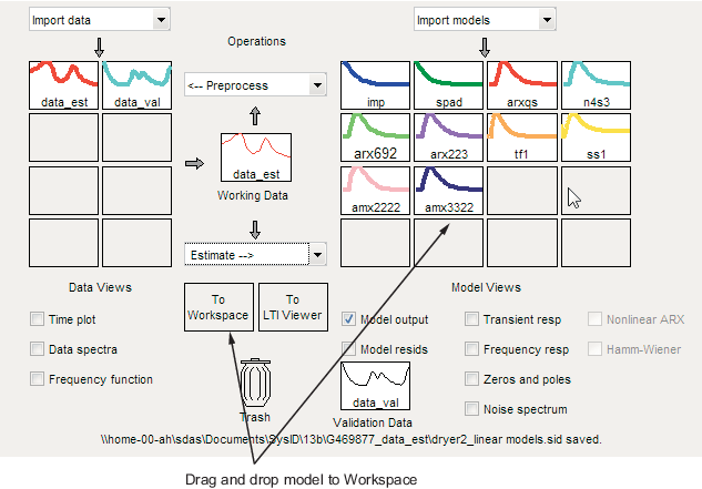
The model appears in the MATLAB Workspace browser.

Note

This model is an idpoly model object.

After the model is in the MATLAB workspace, you can perform other operations on the model. For example, if you have the Control System Toolbox product installed, you might transform the model to a state-space object using:

ss_model=ss(amx3322)

Exporting the Model to the Linear System Analyzer

If you have the Control System Toolbox product installed, the To Linear System Analyzer rectangle appears in the System Identification app.

The Linear System Analyzer is a graphical user interface for viewing and manipulating the response plots of linear models. It displays the following plots:

Step- and impulse-response
Bode, Nyquist, and Nichols
Frequency-response singular values
Pole/zero
Response to general input signals
Unforced response starting from given initial states (only for state-space models)

To plot a model in the Linear System Analyzer, drag and drop the model icon to the To Linear System Analyzer rectangle in the System Identification app. Alternatively, click Show in Linear System Analyzer in the Data/model Info dialog box.

For more information about working with plots in the Linear System Analyzer, see Linear System Analyzer Overview (Control System Toolbox).