impulseest

Estimate a nonparametric impulse response model using data from a hair dryer. The input is the voltage applied to the heater and the output is the heater temperature. Use the first 500 samples for estimation.

Load the data and use the first 500 samples to estimate the model.

load dry2data dry2tt
tte = dry2tt(1:500,:);
sys = impulseest(tte);

tte is a timetable that contains time-domain data. sys, the identified nonparametric impulse response model, is an idtf model.

Analyze the impulse response of the identified model from time 0 to 1.

h = impulseplot(sys,1);

Determine the point at which a significant response to the impulse begins. First, display the region that bounds amplitudes that are not significantly different from zero. To do so, right-click the plot and select Characteristics > Confidence Region. For impulse response plots, by default, this selection displays a confidence region with a width of one standard deviation that is centered at zero, instead of one centered at the response values. You can modify these defaults by right-clicking the plot and selecting Properties > Options.

Alternatively, you can use the showConfidence command.

showConfidence(h);

The first response value that is significantly different than zero occurs at 0.24 seconds, or the third sample. This implies that the transport delay is three samples. To generate a model that imposes the three-sample delay, set the transport delay, which is the third argument, to 3. You must also set the second argument, the order n, to its default value of [] as a placeholder.

sys1 = impulseest(tte,[],3);
h1 = impulseplot(sys1,1);
showConfidence(h1);

The response is identically zero until 0.24 seconds.

Load the estimation data.

load sdata3 umat3 ymat3 Ts;

Estimate a 35th-order FIR model.

n = 35;
sys = impulseest(umat3,ymat3,n);

You can confirm the model order of sys by displaying the number of terms.

nsys = size(sys.num)

nsys = 1×2

     1    35

Set n to [] so that the function automatically determines n. Display the model order.

n = [];
sys1 = impulseest(umat3,ymat3,n);
nsys1 = size(sys1.Numerator)

nsys1 = 1×2

     1    70

The model order is 70. The default value for the order is [], so setting the order to [] is equivalent to omitting the specification.

Estimate an impulse response model with a transport delay of 3 samples.

If you know about the presence of delay in the input/output data in advance, use the delay value as a transport delay for impulse response estimation.

Generate data that contains a 3-sample input-to-output lag.

Create a random input signal. Construct an idpoly model that includes three sample delays, which you implement by using three leading zeros in the B polynomial.

u = rand(100,1);
A = [1 .1 .4];
B = [0 0 0 4 -2];
C = [1 1 .1];
sys = idpoly(A,B,C);

Simulate the model response y to the noise signal, using the AddNoise option and a sample time of 1 second. Encapsulate y in an iddata object.

opt = simOptions('AddNoise',true);
y = sim(sys,u,opt);
data = iddata(y,u,1);

Estimate and plot a 20th order model with no transport delay.

n = 20;
model1 = impulseest(data,n);
impulseplot(model1);

The plot shows that the impulse response includes nonzero samples during the 3-second delay period.

Estimate a model with a 3-sample transport delay.

nk = 3;
model2 = impulseest(data,n,nk);
impulseplot(model2)

The first three samples are identically zero.

Obtain regularized estimates of impulse response model using the regularizing kernel estimation option.

Estimate a model using regularization. impulseest performs regularized estimates by default, using the tuned and correlated kernel ('TC').

load iddata3 z3;
sys1 = impulseest(z3);

Estimate a model with no regularization.

opt = impulseestOptions('RegularizationKernel','none');
sys2 = impulseest(z3,opt);

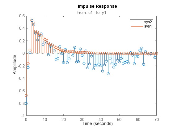
Compare the impulse responses of both models.

h = impulseplot(sys2,sys1,70);
legend('sys2','sys1')

As the plot shows, using regularization makes the response smoother.

Plot the confidence intervals.

showConfidence(h);

The uncertainty in the computed response is reduced at larger lags for the model using regularization. Regularization decreases variance at the price of some bias. The tuning of the 'TC' regularization is such that the variance error dominates the overall error.

Load the estimation data.

load regularizationExampleData eData;

Recreate the transfer function model that was used for generating the estimation data (true system).

num = [0.02008 0.04017 0.02008];
den = [1 -1.561 0.6414];
Ts = 1;
trueSys = idtf(num,den,Ts);

Obtain a regularized impulse response (FIR) model with an order of 70.

opt = impulseestOptions('RegularizationKernel','DC');
m0 = impulseest(eData,70,opt);

Convert the model into a state-space model and reduce the model order.

m1 = idss(m0);
m1 = balred(m1,15);

Estimate a second state-space model directly from eData by using regularized reduction of an ARX model.

m2 = ssregest(eData,15);

Compare the impulse responses of the true system and the estimated models.

impulse(trueSys,m1,m2,50);   
legend('trueSys','m1','m2');

The three model responses are similar.

Use the empirical impulse response to measured data to determine whether the data includes feedback effects. Feedback effects can be present when the impulse response includes statistically significant response values for negative time values.

Compute the noncausal impulse response using a fourth-order prewhitening filter and no regularization, automatic order selection, and negative lag.

load iddata3 z3;
opt = impulseestOptions('pw',4,'RegularizationKernel','none');
sys = impulseest(z3,[],'negative',opt);

sys is a noncausal model containing response values for negative time.

Analyze the impulse response of the identified model.

h = impulseplot(sys);

View the zero-response region at one standard deviation by right-clicking on the plot and selecting Characteristics > Confidence Region. Alternatively, you can use the showConfidence command.

showConfidence(h);

The large response value at t=0 (zero lag) suggests that the data comes from a process containing feedthrough. That is, the input affects the output instantaneously. The large response value can also indicate direct feedback, such as proportional control without some delay so that y(t) partly determines u(t).

Other indications of feedback in the data are the significant response values such as those at -7 seconds and -9 seconds.

Compute an impulse response model for frequency response data.

Load the frequency response data, which contains measured amplitude AMP and phase PHA for the frequency vector W.

load demofr;

Create the complex frequency response zfr and encapsulate it in an idfrd object that has a sample time of 0.1 seconds. Plot the data.

zfr = AMP.*exp(1i*PHA*pi/180);
Ts = 0.1;
data = idfrd(zfr,W,Ts);

Estimate an impulse response model from data and plot the response.

sys = impulseest(data);
impulseplot(sys)

Identify parametric and nonparametric models for a data set, and compare their step responses.

Estimate the impulse response model sys1 (nonparametric) and state-space model sys2 (parametric) using the estimation data set z1.

load iddata1 z1;
sys1 = impulseest(z1);
sys2 = ssest(z1,4);

sys1 is a discrete-time identified transfer function model. sys2 is a continuous-time identified state-space model.

Compare the step responses for sys1 and sys2.

step(sys1,'b',sys2,'r');
legend('Impulse response model','State-space model');