Main Content

Estimate Spectral Model

Estimate spectral model using time-domain data in the Live Editor

Since R2021b

Description

The Estimate Spectral Model task lets you interactively estimate and plot a spectral model using time data. You can specify one of three estimation algorithms and modify the size of the window size that determines frequency resolution. You can also specify the frequency vector, including the number of frequencies and whether those frequencies are evenly spaced on a linear or a logarithmic scale. The task automatically generates MATLAB® code for your live script. For more information about Live Editor tasks in general, see Add Interactive Tasks to a Live Script.

A frequency-response model is the frequency response of a linear system evaluated over a range of frequency values. The model is represented by an idfrd model object that stores the frequency response, sample time, and input-output channel information. For more information about frequency-response models, see What is a Frequency-Response Model?.

The Estimate Spectral Model task is independent of the more general System Identification app. Use the System Identification app when you want to compute and compare estimates for multiple models.

To get started, load experiment data that contains input and output data into your MATLAB workspace and then import that data into the task. Then, specify a model structure to estimate. The task gives you controls and plots that help you experiment with different model parameters and compare how well the output of each model fits the measurements.

Related Functions

The code that Estimate Spectral Model generates uses the following functions.

  • Data objects:

    • iddata — Contains input-output data

  • Algorithms for estimating frequency response:

  • Frequency Plots:

The task estimates an idfrd frequency-response model.

Estimate Spectral Model task in Live Editor

Open the Task

To add the Estimate Spectral Model task to a live script in the MATLAB Editor:

  • On the Live Editor tab, select Task > Estimate Spectral Model.

  • In a code block in your script, type a relevant keyword, such as spectral or estimate. Select Estimate Spectral Model from the suggested command completions.

Examples

expand all

Use the Estimate Spectral Model Live Editor Task to estimate a frequency-response model and plot the response.

Set Up Data

Load the measurement data tt2 into your MATLAB workspace.tt2 is a timetable that contains one input variable u and one output variable y.

load sdata2 tt2

Import Data into Task

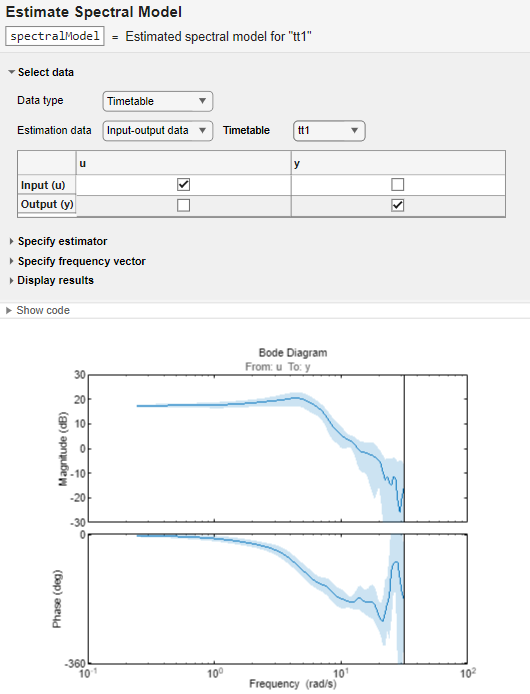
In the Select data section, for Data type, select Timetable. For Estimation data, select Input-output data. In Timetable, select tt2.

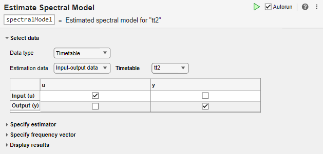
The task displays a table that contains the tt2 input and output variable names.

Estimate Model Using Default Settings

The default algorithm is SPA (Blackman-Tukey).

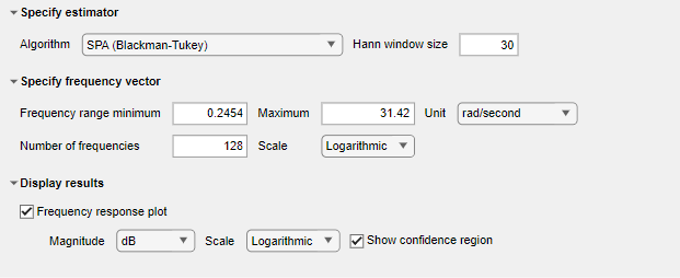
Because Autorun is selected, the task automatically performs the estimation, using this algorithm and the default settings for Specify frequency vector and Display results.
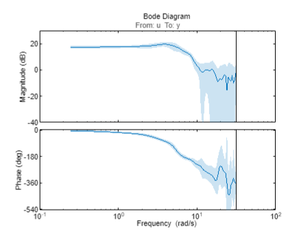
Examine Plot

The task displays a Bode plot that includes a confidence region of three standard deviations.
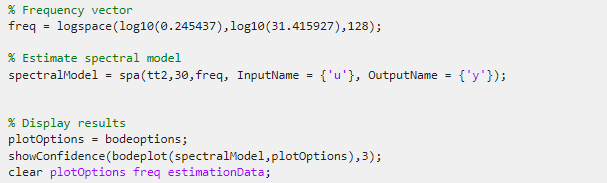
View Code

To display the code that the task generates, click at the bottom of the parameter section. The code that you see reflects the current parameter configuration for the task.

Parameters

expand all

Select Data

The task accepts numeric measurement values that are uniformly sampled in time. Input and output signals can contain multiple channels. Data can be packaged either as numeric arrays (for Numeric), in a timetable (for Timetable), or in an iddata object (for Data object).

The data type you choose determines whether you must specify additional parameters.

  • Numeric — Specify Sample Time in the time units that you select.

  • Timetable — Specify no additional parameters because the timetable already contains information on time sampling.

  • Data Object — Specify no additional parameters because the data object already contains information on time sampling.

The task accepts input-output data and time series data that has no input array.

The estimation data content you select, along with your selection of Data Type, determines your options for accessing variables from your MATLAB workspace.

  • Input-Output Data

    • Numeric data — Select the variable name of the for your input and output vectors for Input (u) and Output (y), respectively.

    • Timetable — When you specify a timetable, the task displays the timetable variables and the default assignment of the variables to input and output signals. You can change these assignments by selecting different variables.

    • Data object — Select the data object.

  • Time series

    • Numeric data — Select the variable name of your output vector for Output (y).

    • Timetable — The task assumes that all the variables in the timetable are output signals and selects them as Output (y). Clear the selections for variables that represent inputs.

    • Data object — Select the data object.

Specify estimator

The task provides three algorithms to choose from.

  • SPA — Blackman-Tukey Spectral analysis (SPA) method. Takes the Fourier transform of windowed versions of the covariance function.

  • SPAFDR — Variant of the SPA method that uses frequency-dependent resolution.

  • ETFE — Empirical transfer function estimate. This method computes the ratio of the Fourier transform of the output to the Fourier transform of the input. For time series, which have no input, this method computes a periodogram as the normalized absolute squares of the Fourier transform of the time series.

For more information on these algorithms, see spa, spafdr, and etfe. For information on selecting an algorithm, see Selecting the Method for Computing Spectral Models.

Each estimation algorithm uses a unique parameter for determining and using the window size.

  • SPAHann window size. Specify this parameter as a positive integer greater than 2. The default value is equal to 30 for data arrays with lengths of 300 or more, or, for smaller arrays, arraylength/10.

  • SPAFDRResolution. Specify this parameter in rad/TimeUnit, where TimeUnit is the unit you specify for Sample Time. The resolution is the size of the smallest detail in the frequency function and the spectrum that is resolved by the estimate. Setting the resolution is a tradeoff between obtaining estimates with fine, reliable details, and suffering from spurious, random effects. The default value in the task is default, which uses the resolution that spafdr calculates based on the frequencies. If you want to view this resolution value for the SISO model spectralModel, at the command line, enter spectralModel.Report.WindowSize.

  • ETFEHamming window size. Specify this parameter, which represents frequency resolution, as a positive integer greater than 2. The value of the parameter determines the amount of smoothing that the function applies to the raw spectral estimates. The default value in the task is default, which uses the resolution that etfe calculates based on the frequencies. If you want to view this resolution value for the SISO model spectralModel, at the command line, enter spectralModel.Report.WindowSize.

Specify frequency vector

Specify the frequency vector minimum and maximum, and select the unit, such as the default rad/second, from the Unit list. By default, the task sets the frequency to span the range bounded at the upper end by the Nyquist frequency, which is a function of the sample time. The task sets the default value of the lower end of the range to the first frequency value.

Specify the number of frequency divisions and whether to use a linear or a logarithmic scale. The default number of divisions is 128. The default scale is Logarithmic.

Display Results

Select Frequency response plot to create a frequency plot of your model. If you specify your data type as Input-output data, then the task creates the frequency response using bode. If your data type is Time series, then the task plots the power spectrum using spectrum.

You can plot only one model at a time in the task. If you want to compare responses, do one of the following:

  • Open multiple tasks and visually compare plots for different models.

  • Use unique model IDs for each model you want to compare, and then create Bode plots for them at the command line.

Specify the parameters for the Bode or power spectrum plot. You can specify that the units in Magnitude are dB or absolute value. For Scale, you can specify a logarithmic or a linear scale for the frequency axis. If you are creating a Bode plot by using input-output data, you can select Show confidence region to display a confidence region of three standard deviations. If you are creating a power spectrum plot by using a time series, no Show confidence region option exists.

Version History

Introduced in R2021b

expand all