Main Content

etfe

Estimate empirical transfer functions and periodograms

Description

g = etfe(data) estimates a transfer function of the form:

y(t)=G(q)u(t)+v(t)

data contains time-domain or frequency-domain input/output data or time series data. data can be in the form of a timetable, comma-separated pair of numeric matrices, or time-domain or frequency-domain iddata object.

  • If data contains time-domain input/output signals, then g is the ratio of the output Fourier transform to the input Fourier transform for the data.

    For nonperiodic data, the transfer function is estimated at 128 equally-spaced frequencies [1:128]/128*pi/Ts.

    For periodic data that contains a whole number of periods (data.Period = integer ), the response is computed at the frequencies k*2*pi/period/Ts for k = 0 up to the Nyquist frequency (pi/Ts), where Ts is the data sample time. The software removes the frequency points where the input signal has insignificant energy from the result.

  • If data contains frequency-domain input/output signals, g is the ratio of output to input at all frequencies, where the input is nonzero.

  • If data contains time-series data (no input channels), g is the periodogram, that is, the normed absolute square of the Fourier transform, of the data. The corresponding spectral estimate is normalized, as described in Spectrum Normalization and differs from the spectrum normalization in the Signal Processing Toolbox™ product.

If data is a timetable, the software interprets the last variable is the single output variable. To change this interpretation, use the InputName and OutputName name-value arguments.

example

g = etfe(data,M) applies a smoothing operation on the raw spectral estimates using a Hamming Window that yields a frequency resolution of about pi/M. The effect of M is similar to the effect of M in spa. M is ignored for periodic data. Use this syntax as an alternative to spa for narrowband spectra and systems that require large values of M.

example

g = etfe(data,M,N) specifies the frequency spacing N for nonperiodic data.

  • For nonperiodic time-domain data, N specifies the frequency grid [1:N]/N*pi/Ts rad/TimeUnit. When not specified, N is 128.

  • For periodic time-domain data, N is ignored.

  • For frequency-domain data, the N is fmin:delta_f:fmax, where [fmin fmax] is the range of frequencies in data, and delta_f is (fmax-fmin)/(N-1) rad/TimeUnit. When not specified, the response is computed at the frequencies contained in data where input is nonzero.

example

g = etfe(___,Name,Value) uses additional model options specified by one or more name-value arguments.

For example, specify the input and output signal variable names using g = etfe(data,'InputName',["u1","u3"],'OutputName',["y1","y4"]).

You can use this syntax with any of the previous input-argument combinations.
Examples

collapse all

Load estimation data.

load sdata1 tt1;

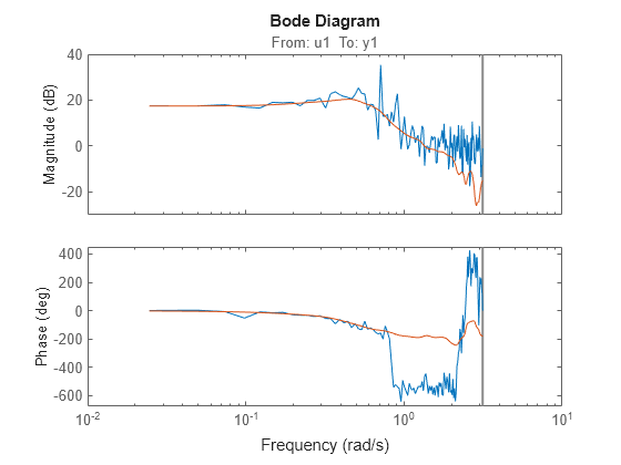
Estimate empirical transfer function and smoothed spectral estimate.

ge = etfe(tt1);
gs = spa(tt1);

Compare the two models on a Bode plot.

bode(ge,gs)

MATLAB figure

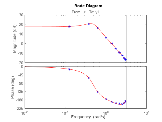
Generate a periodic input, simulate a system with it, and compare the frequency response of the estimated model with the original system at the excited frequency points.

Generate a periodic input signal and output signal using simulation.

m = idpoly([1 -1.5 0.7],[0 1 0.5]);
u = iddata([],idinput([50,1,10],'sine'));
u.Period = 50;
y = sim(m,u);

Estimate an empirical transfer function.

me = etfe([y u]);

Compare the empirical transfer function with the original model.

bode(me,'b*',m,'r')

MATLAB figure

Perform a smoothing operation on raw spectral estimates using a Hamming Window and compare the responses.

Load data.

load sdata1 umat1 ymat1

Estimate empirical transfer functions with and without the smoothing operation.

ge1 = etfe(umat1,ymat1);
ge2 = etfe(umat1,ymat1,32);

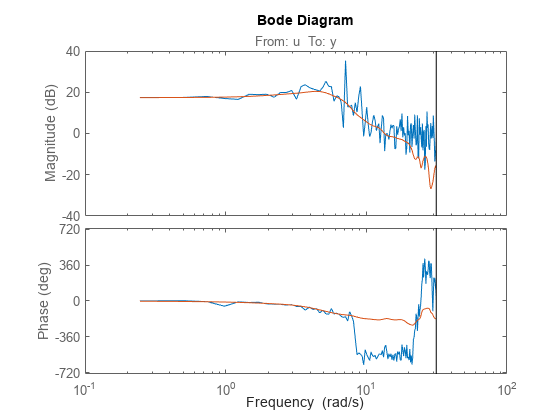
Compare the models on a Bode plot.

ge2 is smoother than ge1 because of the effect of the smoothing operation.

bode(ge1,ge2)

MATLAB figure

Estimate empirical transfer functions with low- and high-frequency spacings and compare the responses.

Load data.

load iddata9

Estimate empirical transfer functions with low and high frequency spacings.

ge1 = etfe(z9,[],32);
ge2 = etfe(z9,[],512);

Plot the output power spectrum of the two models.

spectrum(ge1,'b.-',ge2,'g')

Figure contains an axes object. The axes object with title From: e@y1 To: y1, ylabel Power (dB) contains 2 objects of type line. These objects represent ge1, ge2.

Input Arguments

collapse all

Uniformly sampled estimation data, specified as a timetable, comma-separated matrix pair, time-domain or frequency-domain iddata object, cell array of timetables, or cell array pair of matrices, as the following sections describe.

Timetable

Specify data as a timetable that uses a regularly spaced time vector. data contains variables representing input and output channels.

For multiexperiment data, specify data as an Ne-by-1 cell array of timetables, where Ne is the number of experiments. The sample times of all the experiments must match.

When you use timetables for estimation, you can use all the variables or specify a subset of channels to use. To select individual input and output channels to use for estimation, use the InputName and OutputName name-value arguments.

For time series data, either specify data as a single-variable timetable containing only an output variable, or use InputName and OutputName name-value arguments to specify only output variables for estimation.

For example, sys = etfe(data,'OutputName',"y2",'InputName',[]) estimates the time series model sys from the timetable data using the output variable y2 and no input variables.

Comma-Separated Matrix Pair

Specify data as a comma-separated pair of matrices u,y that contain uniformly sampled input and output time-domain signal values. Matrix-based data provides no sample-time information. The software assumes that the sample time is one second. Using matrix-based data for continuous-time systems is not recommended.

For SISO systems, specify u,y as column vectors with a length of Ns, where Ns is the number of samples.

For MIMO systems, specify u,y as a matrix pair with the following dimensions:

  • uNs-by-Nu, where Nu is the number of inputs

  • yNs-by-Ny, where Ny is the number of outputs

For multiexperiment data, specify u,y as a pair of 1-by-Ne cell arrays, where Ne is the number of experiments.

For time series systems, specify an empty u, that is, [],y.

Data Object

An estimation data object, specified as a time-domain or frequency-domain iddata object that contains uniformly sampled input and output values. The data object can have one or more output channels and zero or more input channels. By default, the software sets the sample time of the model to the sample time of the estimation data.

For more information about working with estimation data types, see Data Domains and Data Types in System Identification Toolbox.

Frequency resolution, specified as a positive scalar. The default value, [] implies that the software does not apply any smoothing operation on the raw spectral estimates.

For more information about working with estimation data types, see Data Domains and Data Types in System Identification Toolbox.

Frequency spacing, specified as a positive scalar. For frequency-domain data, the default frequency spacing is the spacing inherent in the estimation data.

Name-Value Arguments

Specify optional pairs of arguments as Name1=Value1,...,NameN=ValueN, where Name is the argument name and Value is the corresponding value. Name-value arguments must appear after other arguments, but the order of the pairs does not matter.

Before R2021a, use commas to separate each name and value, and enclose Name in quotes.

Example: sys = etfe(data,'InputName',"u2")

Input channel names, specified as a string, character vector, string array, or cell array of character vectors.

If you are using a timetable for the data source, the names in InputName must be a subset of the timetable variables.

Example: sys = etfe(tt,__,'InputName',["u1" "u2"]) selects the variables u1 and u2 as the input channels from the timetable tt to use for the estimation.

Output channel names, specified as a string, character vector, string array, or cell array of character vectors.

If you are using a timetable for the data source, the names in OutputName must be a subset of the timetable variables.

Example: sys = etfe(tt,__,'OutputName',["y1" "y3"]) selects the variables y1 and y3 as the output channels from the timetable tt to use for the estimation.

Sample time, specified as the comma-separated pair consisting of 'Ts' and the sample time in the units specified by TimeUnit. When you use matrix-based data (u,y), you must specify Ts if you require a sample time other than the assumed sample time of 1 second.

To obtain the data sample time for a timetable tt, use the timetable property tt.Properties.Timestep.

Example: etfe(umat1,ymat1,___,'Ts',0.08) computes a model with sample time of 0.08 seconds.

Output Arguments

collapse all

Transfer function estimate, returned as an idfrd model.

Information about the estimation results and options used is stored in the model's Report property. Report has the following fields:

Report FieldDescription
Status

Summary of the model status, which indicates whether the model was created by construction or obtained by estimation

Method

Estimation command used

WindowSize

Size of the Hamming window.

DataUsed

Attributes of the data used for estimation, returned as a structure with the following fields.

  • Name — Name of the data set

  • Type — Data type

  • Length — Number of data samples

  • Ts — Sample time

  • InterSample — Input intersample behavior, returned as one of the following values:

    • 'zoh' — A zero-order hold maintains a piecewise-constant input signal between samples.

    • 'foh' — A first-order hold maintains a piecewise-linear input signal between samples.

    • 'bl' — Band-limited behavior specifies that the continuous-time input signal has zero power above the Nyquist frequency.

  • InputOffset — Offset removed from time-domain input data during estimation. For nonlinear models, it is [].

  • OutputOffset — Offset removed from time-domain output data during estimation. For nonlinear models, it is [].

For more information on using Report, see Estimation Report.

Version History

Introduced before R2006a

expand all