spectrum
绘制或返回时间序列模型的输出功率谱或线性输入/输出模型的扰动谱
语法
说明
绘制结果
spectrum( 绘制辨识的时间序列模型 sys)sys 的输出功率谱或辨识的输入/输出模型 sys 的扰动谱。该函数自动选择频率范围和点数。
如果
sys是时间序列模型,则sys代表系统:这里,e(t) 是高斯白噪声,y(t) 是观察到的输出。
spectrum图 |H'H|,按 e(t) 的方差和采样时间缩放。如果
sys是输入/输出模型,则sys代表系统:这里,u(t) 是测量输入,e(t) 是高斯白噪声,y(t) 是观察到的输出。
在这种情况下,
spectrum绘制了干扰分量 He(t) 的频谱。
对于采样时间为 Ts、spectrum 的离散时间模型,使用变换 将单位圆映射到实频率轴。该函数仅绘制小于奈奎斯特频率 π/Ts 的频率的频谱,并且在未指定 Ts 时使用 1 个时间单位的默认值。
示例
加载时间序列估计数据。
load iddata9 z9
使用最小二乘法估计四阶 AR 模型。
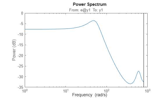
sys = ar(z9,4,'ls');绘制模型的输出频谱。
spectrum(sys);
要更改图中的显示选项,右键点击该图以访问上下文菜单。例如:
要查看仿真响应的置信域,请选择 Characteristics > Confidence Region。
要指定要绘制的标准差数,请选择 Properties。然后,在属性编辑器中,选择 Options 选项卡,并在 Number of standard deviations for display 中指定标准差数。默认值 1 个标准差。
加载估计数据。
load iddata1 z1;
估计单输入单输出状态空间模型。
sys = n4sid(z1,2);
绘制模型的噪声频谱。指定频率范围从 0.1 到 50 弧度/秒。
spectrum(sys,{0.1,50});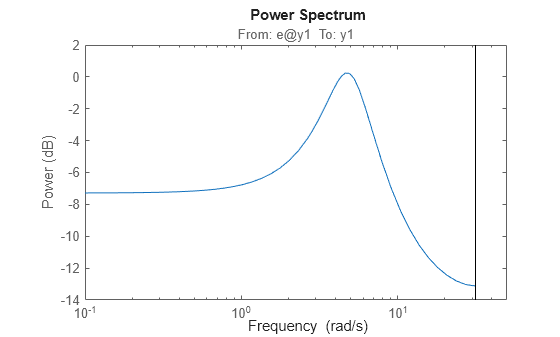
该函数绘制频谱,但将频率范围限制为奈奎斯特频率约 31.4 rad/s。
创建一个由五个正弦波的总和组成的输入,每个正弦波分布在整个频率范围内。将该信号的频谱与其平方的频谱进行比较。
创建一个延续 20 个周期的正弦波总和输入,每个周期包含 100 个采样。指定信号组合 5 个随机相位的正弦波,使用 10 次试验来找到信号扩散最低的集合。有关此步骤的详细信息,请参阅 idinput。
u = idinput([100 1 20],'sine',[],[],[5 10 1]);创建一个仅输入的 iddata 对象 u,其中包含输入 u 且周期为 100。
u = iddata([],u,1,'per',100);对输入值进行平方并将其存储在新的 iddata 对象 u2 中。
u2 = u.u.^2;
u2 = iddata([],u2,1,'per',100);
使用 etfe 从 u 和 u2 估计经验传递函数模型。将这些模型的功率谱绘制在一起。使用不同的标记颜色和类型来区分频谱源。
spectrum(etfe(u),'r*',etfe(u2),'+')
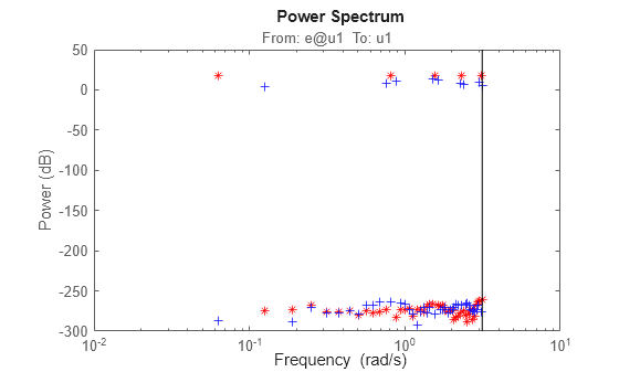
该图显示了一些频率分裂,其中基于 u2 的频谱与基于 u 的频谱不一致,而是包含两个与某些基于 u 的点相邻的频谱点。这种分裂表明了平方系统的非线性。
输入参数
输出参量
版本历史记录
在 R2012a 中推出